 By Gustavo Torres
If you have ever built a semantic search engine, you chose the cosine without choosing it. A search engine like that turns every text into an embedding, a vector of numbers with which a model represents it, and compares the question with each document using cosine similarity: the cosine of the angle between the two vectors. It is when they point the same way and drops the further apart they are, and the engine returns the texts with the highest value. It is the default in almost every vector database (the ones that store vectors and return those most similar to a given one), the measure OpenAI recommends for its embeddings, and the one that RAG tutorials take for granted (retrieval-augmented generation: finding the passages most similar to a question and handing them to the model so it answers with them).
Many libraries, though, don't give you the similarity but its reverse, one minus the cosine, so
that a smaller value means "closer", as with any distance. SciPy, Python's scientific library, calls
it
"Cosine distance".
In pgvector, PostgreSQL's vector extension, it is what the
<=> operator returns. In scikit-learn, the machine learning library, you ask for it with
metric="cosine". Sorting from smallest to largest is the same as sorting
from largest to smallest, so the search returns the same results either way. What
changes is the name: the similarity, turned inside out, is presented as a distance, and in
scikit-learn even as a metric.
Take three vectors of length one leaving the same point. A points horizontally, C vertically and B right in between, at 45°. The cosine distance, , is between A and B, and another between B and C. Between A and C it is . Going from A to C through B costs , and going straight costs .
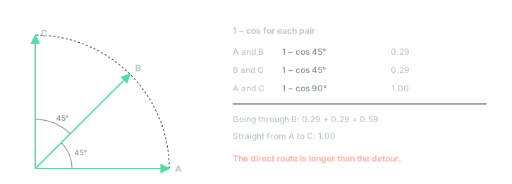
Three vectors and the cosine distance: the direct route is longer than the detour.
No distance worth the name allows that. The direct route can't be longer than a detour: that is the triangle inequality, and the cosine distance does not satisfy it. So there are two things worth keeping apart. Cosine similarity, the one that ranks the results, is not a distance: it is a score of resemblance. And the cosine distance built from it is not a metric.
And yet the cosine is the right choice almost every time. There are two questions. The first is why it has won among the dozens of ways there are to compare two vectors. The second is what it costs that its distance isn't a metric, which in a search is nothing and in other operations is quite a lot. Along the way come the measures it competes with and the cases where it stops being the right tool.
An embedding is a vector
An embedding is a vector with which a model represents a piece of text: a word, a sentence, a whole document. A vector of dimensions is numbers, and current models use hundreds or thousands (384, 768, 1,536 and 3,072 are common sizes). The model is trained so that texts that mean something similar get similar vectors. A vector of numbers is a point in a -dimensional space, and it is usually drawn as an arrow that leaves the origin and ends at that point.
Two of a vector's properties matter here. The first is its length, or norm:
The second is its direction, where it points.
To compare two vectors, the basic tool is the dot product: multiply coordinate by coordinate and add up. It has a geometric reading that connects it with the angle between the two:
Solving for the cosine gives cosine similarity:
It is when the two vectors point the same way, when they are perpendicular and when they point in opposite directions. And it doesn't change if you stretch or shrink either of them: dividing by the lengths is precisely removing them. The vectors and have cosine , even though the second is twice as long and the distance between their tips is .
That distance between the tips is the other classic comparison, the Euclidean distance: , the length of the vector that goes from one tip to the other. It sees direction and length at once. The cosine sees only the direction, and whatever was stored in the length it throws away. That discarding is the whole story: why it is almost always right, and what it costs.
Similarity, distance and metric
Three words used as synonyms that name three different things.
A similarity is any score that grows the more two things resemble each other. It promises nothing else: not a maximum value, not even that a thing is most similar to itself. The cosine is a similarity.
A distance, in the broad sense that libraries use, is the opposite: a score that grows the more they differ. Any similarity becomes one by flipping it, and is the "cosine distance" of SciPy and pgvector. It goes from (same direction) to (opposite directions).
A metric is a distance that obeys four rules. Here the word has its geometric sense, not the sense of evaluation metrics such as a classifier's accuracy. For any , , :
- . No distance is negative.
- only if . Distance zero means "they are the same".
- . It doesn't matter where you measure from.
- . The triangle inequality: the direct route is never longer than a detour.
The fourth does the most work. It says that knowing two distances bounds the third: if is close to and is close to , can't be far from . Everything that reasons with distances without computing them all relies on it.
Now, rule by rule. It meets the first, because the cosine never exceeds . The third too, because the angle from to is the same as from to . The second fails: and are different vectors and their cosine distance is . At best it compares directions, not vectors. This one has an easy fix: if before anything else you divide each vector by its length (which is called normalising: making them all length one), two vectors with the same direction are the same vector.
The fourth fails even then, and it is the opening example. The three vectors have length one, and . The detour adds up to and the direct route measures .
So is a distance in the broad sense and not a metric. The plain cosine isn't even a
distance: it is a similarity. With this vocabulary, the library names from the opening read better.
SciPy and pgvector are right to call a distance, in the broad sense. scikit-learn
asks for it with a parameter called metric, but there the word only means "comparison function",
not the four rules. The one that says it outright is FAISS, Meta's library for searching among
millions of vectors: its
documentation makes clear
that the cosine is a similarity and not a distance, and it doesn't even offer it as an option. To
search by cosine, you normalise the vectors and search by dot product (METRIC_INNER_PRODUCT).
Two true metrics with the same order
The cosine hides two true metrics, and both appear when you normalise. If and are and divided by their length, their tips lie on the sphere of radius one and the cosine is simply their dot product: .
The first is the angle, . On the sphere of radius one, the angle is the length of the shortest arc between the two tips without leaving the surface, the route a plane flies between two cities. That distance does satisfy the triangle inequality: with the three vectors, . The detour through B ties with the direct route, because B lies right in the middle of the way, and it never beats it.
The second is the chord, the Euclidean distance between the normalised vectors. Its relation to the cosine takes one line, expanding the square and using :
So , which is a metric because the Euclidean distance is.
Read backwards, the same identity explains the failure from the opening:
The "cosine distance" is half the square of the Euclidean distance between the normalised vectors. And squaring breaks the triangle inequality. On a line, the points , and are at distances , and ; squared, , and , and . Squaring penalises large distances more than small ones, so one long trip costs more than two half trips. With small angles you can see it in numbers: , and two steps of cost each, together, while the in one go cost , twice as much.
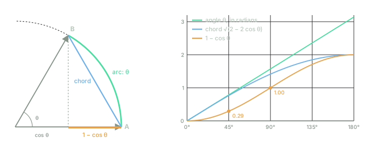
Three ways of measuring how far apart two directions are. The arc and the chord are metrics; 1 − cos starts flat, which is why two short steps add up to less than one long one.
The important consequence is in the right-hand chart: the three measures always grow with the angle. Larger angle, larger chord, larger and smaller cosine go together, so all three rank any list of candidates exactly the same way. Searching for the ten closest texts by cosine, by angle or by Euclidean distance between normalised vectors gives the same ten, in the same order. It is what OpenAI's guide says: its embeddings come normalised, so cosine and Euclidean distance produce the same ranking.
For searching, which is what the cosine is used for almost always, not being a metric doesn't matter at all. It matters when you do something with the numbers other than sorting them.
When it does matter
There are three situations: when an algorithm uses the triangle inequality to save computations, when vectors are averaged, and when similarities are chained.
Indexes that discard without looking
Some exact nearest-neighbour indexes, such as the ball tree, group the points into balls with a centre and a radius, and discard a whole ball with a single computation. If the query is at distance from the centre and the ball has radius , everything inside is at least from the query, by the triangle inequality. If already exceeds the best candidate found so far, the ball is skipped without looking inside. With a distance that doesn't satisfy the inequality, that bound is false and the index would discard true neighbours.
scikit-learn knows. Neither its BallTree nor its KDTree accepts the cosine, and when you ask for
NearestNeighbors(metric="cosine") with the automatic algorithm,
it falls back to brute force: comparing the
query with everything. The fix is the previous section. Normalise the vectors, ask for the Euclidean
distance, and the tree works with the same order.
Graph indexes such as HNSW (Hierarchical Navigable Small World, the one many vector databases use) don't discard with the triangle inequality. They walk a graph of neighbours, always jumping to the most promising one, and they are approximate anyway. That is why hnswlib, the open-source library maintained by HNSW's first author, offers the dot product and the cosine alongside the Euclidean distance, with a warning that the dot product is not a metric.
Averaging
k-means groups points into clusters by repeating two steps: assign each point to the nearest centre and move each centre to the mean of its points. It is built for the Euclidean distance, and with directions the mean has a catch: the mean of length-one vectors doesn't have length one. Two perpendicular vectors, and , average to , of length , and the more spread out a cluster is, the shorter its centre.
If you run plain k-means on normalised vectors, the assignment step compares each point with centres of different lengths. Since , the last term favours the clusters with the shortest centre, the most spread out ones, for a reason that has nothing to do with resemblance. Spherical k-means (Dhillon and Modha, 2001) fixes it by normalising each centre again after averaging. The same goes for any average of embeddings: the mean of normalised vectors has to be normalised again before comparing it with anything.
Chaining
"A resembles B and B resembles C, so A resembles C." It is the reasoning of anyone who deduplicates a corpus, clusters by chains or recommends friends of friends. With a metric, the conclusion has a bound. With the cosine too, if you go through the angle, which is a metric.
Suppose and , with . Each of the two angles measures at most . By the triangle inequality for angles,
The cosine decreases between and , so a larger angle gives a smaller cosine, and the double-angle formula, , finishes the calculation:
With , is guaranteed. With , . With , : nothing. A and C can be perpendicular, unrelated, even though each step looks fairly similar. The bound is tight, because it is reached when B lies right in the middle of the arc between A and C, which is what happened with the three vectors: and .
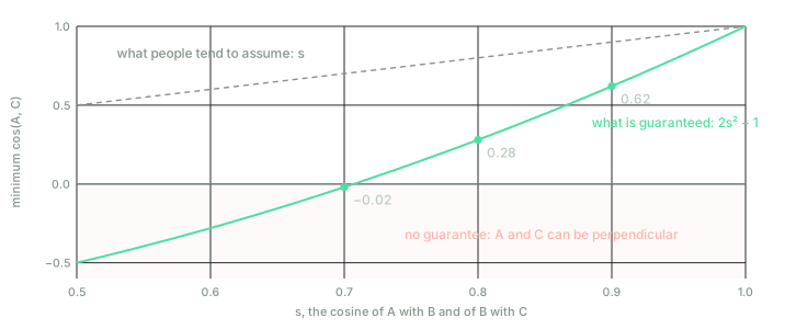
What two similarities guarantee about the third. Below 0.71 per step, nothing.
A threshold of for "similar" doesn't compose. Two hops of can join texts that have nothing to do with each other, and a clustering method that merges groups through chains (single linkage) with that threshold ends up connecting anything with anything, given enough intermediate steps.
Why the cosine won
If the cosine, the angle and the Euclidean distance between normalised vectors rank the same way, the question is not why the cosine rather than the Euclidean distance. It is why throw the length away. There are four reasons, and a fifth that gets repeated a lot and doesn't hold up.
The legacy of information retrieval
In 1975, Salton, Wong and Yang described the vector space model for searching documents: each document is a vector with one coordinate per term, weighted by its importance (what would later be called TF-IDF, term frequency–inverse document frequency: how many times the word appears in the document times how rare it is in the collection). On the first page they already propose comparing documents by the angle between their vectors, and normalising them all to length one to put them on the sphere.
The reason was practical. A long document repeats more words, so its vector is longer, and with the dot product long documents would win any search just for being long. The cosine removes the length, which there was an accident of the text and not of its topic. When word2vec arrived in 2013, the first popular word-vector model, the habit came with it: its authors already solved analogies by looking for the closest word "measured by cosine distance". Language processing inherited the measure from search engines.
Length measures something else
In word vectors, length isn't meaning. Schakel and Wilson studied it in 2015 with word2vec, and it turned out to mix two things: how frequent a word is and how consistent the context it appears in is. A word that always shows up in the same kind of sentence gets a longer vector the more often it appears. One that shows up in very different contexts, like "the" or "of", ends up with a short vector, because each context pulls it in a different direction and the pulls cancel out. They propose using the length to measure how much a word matters in a corpus. It is useful information, but it isn't resemblance: with the dot product, two words would come out closer for being important, not for meaning the same thing. The cosine only asks where each vector points.
Models are trained with the cosine
It is the strongest reason today, and it is circular in the good sense: embedding models are trained with the cosine inside the loss function. Sentence-BERT (2019), the model that popularised sentence embeddings, promised in its abstract vectors that can be compared with the cosine. Contrastive training, today's standard, pulls together the pairs that should be similar and pushes the rest apart, measuring with the cosine divided by a temperature, a number that sets how hard the contrast is: in SimCSE, a contrastive method from 2021. Wang and Isola (2020) formalised it: the vectors are placed on the sphere of radius one and training seeks two things, alignment (similar pairs together) and uniformity (everything else spread over the whole sphere).
A model trained like that never received any signal about length, because the loss didn't see it. Length is noise, and many models remove it themselves: OpenAI's embeddings come out already normalised. With them, the cosine, the dot product and the Euclidean distance are interchangeable, and the dot product is the cheapest. The general rule is that the right measure is the one used to train the model.
It is cheap
You normalise once, at indexing time, and from then on each cosine is a dot product: multiplications and additions. Comparing a query with a million documents is a single matrix-vector product, the operation graphics cards and linear algebra libraries do best. Since the result lives between and , the vectors compress well, for example to 8-bit integers.
And the angle has its own shortcut. Charikar showed in 2002 that if you cut space with a random plane through the origin, the probability that two vectors fall on different sides is . With 256 random planes, each vector becomes 256 bits, and the fraction of bits in which two vectors differ estimates their angle divided by . It is called SimHash, and it estimates the angle, the metric, not .
What doesn't explain it: the curse of dimensionality
A common explanation is that in many dimensions the Euclidean distance loses its meaning and the cosine doesn't. The first half has a basis: Beyer and others proved in 1999 that, under fairly general conditions, as the dimension grows the point nearest to a query and the farthest one end up at almost the same distance. The second half can't be true with normalised vectors: if the cosine and the Euclidean distance rank the same way, they suffer the same.
The cosine concentrates too. Between two random directions in dimensions, the cosine has mean and standard deviation . In 768 dimensions that is , so almost every pair of random vectors is almost perpendicular. What saves embeddings is not the measure: it is that their points aren't random, but crowded into a small, structured part of the space.
So the underlying choice is whether to keep the length or throw it away. In almost all text embeddings the length is noise (the model never learnt to use it) or measures something we don't want to compare (how frequent or important a word is, how long a document is). That's why the cosine.
The other measures
The table sums up the ones that appear in language processing, what they are and whether they see length.
| measure | what it is | sees length? | where it appears |
|---|---|---|---|
| cosine | similarity, from to | no | almost every text embedding model |
| angle, | metric | no | SimHash; when a true metric is needed |
| dot product | unbounded similarity | yes | DPR, recommender systems |
| Euclidean | metric | yes, except between normalised vectors | tree indexes, k-means |
| Manhattan | metric: sum of absolute differences | yes | rarely with embeddings |
| Mahalanobis | metric that discounts the correlations between coordinates | yes | whitening embeddings |
| Pearson | similarity, from to | no | the cosine after subtracting from each vector the mean of its coordinates |
| Jaccard | is a metric; compares sets | n/a | deduplicating corpora (with MinHash) |
| Hamming | metric: counts differing bits | n/a | binary codes, SimHash |
| Jensen–Shannon | divergence between distributions; its square root is a metric | n/a | comparing word or topic distributions |
| cross-encoder | learnt, no geometry | n/a | reranking results |
Three deserve a paragraph.
The dot product is the one that keeps the length, and it is the right one when length is information. In a recommender system, the product of a user's vector and an item's vector is the prediction, and the length of an item's vector tends to capture how popular it is, which is a good reason to recommend it. DPR (Dense Passage Retrieval, 2020), a passage retriever for answering questions, was trained with the dot product, and in its own tests the Euclidean distance performed similarly and both beat the cosine, though with settings chosen for the dot product. That said, it isn't even a well-behaved similarity: a vector can resemble another more than it resembles itself. With and , the product of the first with itself is and with the second is .
The Mahalanobis distance is the Euclidean one after whitening the data: transforming it so that the coordinates are uncorrelated and all have the same variance. It is the link to the fix in the next section.
Cross-encoders play a different game. All the measures above compare two vectors computed separately, each text encoded on its own. A cross-encoder reads both texts at once and returns a score, so it sees each word of one against each word of the other, and it is usually more accurate. The price is that nothing can be computed in advance: each pair is a full pass of the model. That's why the usual pattern is to use the cosine to pull a hundred candidates out of millions, and the cross-encoder to rerank those hundred. The cosine isn't the best similarity there is. It's the best one that fits in an index.
Where the cosine doesn't fit
First, a distinction that saves arguments: a failure of the measure is not the same as a failure of the representation. "Hot" and "cold" have a high cosine in many word models, and so do a sentence and its negation. That isn't the cosine's fault. Those words appear in the same contexts, the model placed them close together, and the cosine faithfully reports what the model learnt. No measure fixes a representation that doesn't tell two things apart; that gets fixed in training.
The failures that do belong to the measure are three.
When everything points the same way
Ethayarajh measured in 2019 the average cosine between randomly chosen words inside language models such as BERT (Google, 2018) and GPT-2 (OpenAI, 2019), taking the vector that each layer of the model gives each word. In GPT-2 it was around in layers 2 to 8, and in the last one almost : any two words had an almost perfect cosine. In BERT's last layer, around . This is called anisotropy: the vectors don't fill the whole sphere but a narrow cone, and everything resembles everything.
Timkey and van Schijndel found part of the cause in 2021: a few rogue dimensions with huge values. In BERT's layer 11, a single coordinate out of 768 contributes 88% of the expected cosine between two vectors; in XLNet, another 2019 model, 99.6%. There the cosine measures one coordinate.
This happens above all when you take vectors out of a language model that wasn't trained to compare them. The fixes, from cheapest to most expensive: centring (subtracting the collection's mean from every vector; Mu and Viswanath also remove the few dominant directions), standardising each coordinate, which is Timkey and van Schijndel's fix, whitening (comparing, at bottom, with the Mahalanobis distance), or using a model trained with a contrastive loss, whose uniformity pushes right against the cone.
Even good models have their own scale. The model card for E5, a family of embedding models, warns that its cosines usually fall between and because of its training temperature (), and that what matters is the relative order. A cosine of doesn't mean "80% similar", and a threshold chosen for one model doesn't work for another: it has to be calibrated with labelled pairs from your own data.
When the length was the signal
Steck, Ekanadham and Kallus, from Netflix, published a paper in 2024 whose title is a question: Is Cosine-Similarity of Embeddings Really About Similarity? In a family of linear recommendation models, the prediction is the product of two matrices, , and you can multiply each column of by any factor and divide the matching column of by the same factor. With a diagonal matrix :
The predictions don't change; the cosines between the rows of do. The model doesn't determine them, and depending on the training they can come out arbitrary. The authors' recipe: if you are going to compare with the cosine, train with the cosine inside the loss. If not, the only thing the model pinned down is the dot product. It is the principle from before, seen from the side where it fails.
When the relation has a direction
The cosine is symmetric: that's the third rule, the one it does satisfy. Many relations aren't. A question and its answer are not interchangeable. A dog is an animal, but not the other way round. A sentence can imply another without the second implying the first.
There are three ways out. Put the asymmetry in the model rather than in the measure: E5 asks you to
prefix questions with query: and documents with passage: , so the same text is encoded
differently depending on its role. Change the geometry:
order embeddings represent "is a" as an order between vectors,
and hyperbolic embeddings place hierarchies in a space where trees
fit without squeezing. Or compare piece by piece: ColBERT, a
retriever from 2020, stores one normalised vector per word and scores by adding up, for each word of
the question, its best cosine with any word of the document. That sum runs over the question and not
the document, so it is asymmetric by construction. And there's always the cross-encoder.
What to take away
If you take away only one thing, let it be this: the cosine is a similarity, and is a distance that isn't a metric, because it is half the square of the Euclidean distance between the normalised vectors. For searching it makes no difference, because the angle, the chord and the cosine rank exactly the same way. For averaging, chaining or pruning an index it does, and the metric to use is the angle or the Euclidean distance between normalised vectors.
And if you take away a second: the cosine didn't win by measuring meaning better, but because it throws the length away, which in almost all text embeddings is noise or measures something else, and because models are trained with it inside the loss.
The rest is practical.
Use the measure the model was trained with. It is usually on its model card. If it's the cosine and the vectors already come normalised, use the dot product: same order, fewer operations.
If the length means something, don't throw it away. Popularity, frequency, importance: if the model was trained with the dot product, compare with the dot product.
Don't set thresholds by eye. A cosine of means different things in each model, and two similarities of don't guarantee a third. Calibrate with labelled pairs and, if you take vectors from a model that wasn't trained to compare them, centre them first.
For relations with a direction, put the asymmetry somewhere else. Different prefixes for questions and documents, or a cross-encoder that reranks the top results.