Attention as query, key and value

28 min read

The block has built a complete mechanism and two different ways of filling its one empty slot: the additive score and the multiplicative one. What it hasn't yet done is stop to look at the vocabulary all of that is written in. Every equation of the last three lessons talks about an encoder that reads, a decoder that writes, states with a bar and states without one. That vocabulary comes from one particular machine (two recurrent networks chained together to translate), and this lesson asks how much of it attention actually needs.

Do it the blunt way: cross out of the equations everything that talks about recurrence and see what's left standing. What remains is a vector that asks, a list of vectors it's compared against, and a list of vectors that get mixed, with a softmax between the two lists and a weighted sum at the end. Not one of those pieces mentions a recurrence, a language or a translation. They're three roles and one operation, each with a name that was fixed years ago and an initial that the next block puts in every one of its equations, starting from the first line of the paper that introduced them.

You've already written an operation that does almost exactly this. In the challenges of the lesson on the long short-term memory (LSTM)Block 3 · Lesson 5LSTM: gated memoryA second state that moves forward by adding rather than by passing through a matrix, and three gates that decide what's kept, what's written and what comes out. Each gate arrives to fix a specific failure of the version before it, and the additive path changes the product that kills the gradient: instead of a power of the recurrent matrix, it becomes a product of numbers the network chooses coordinate by coordinate and can hold at one. and the lesson on the gated recurrent unit (GRU)Block 3 · Lesson 6GRU: the simplified versionAn update gate that ties keeping to writing (whatever isn't kept is exactly what gets written), a reset gate that lets the candidate ignore the past, and one state instead of two. It needs three quarters of the LSTM's weights, and the return path survives, because the direct path still multiplies by a number the network chooses and can hold close to one., the weights arrived in a dictionary P, and you took each piece out with something like P["z"]. You give a query, Python compares it with the stored keys and hands back the value of the one that matches. Get one letter wrong and there's no answer.

Attention is that lookup with the requirement to match taken away. The query doesn't have to equal any key: it's compared with all of them, each comparison becomes a weight, and what comes back isn't one value but a mixture of all of them, each in the proportion its weight gives it. A dictionary returns one of its values; attention returns a combination of all of them. So far in this block, the three roles have been dealt out like this: the decoder state asks, and each source position supplies the other two, what the query is compared with and what gets poured into the mixture.

Three roles, three arguments

Take the three roles as three objects, without saying where they come from: a query $\mathbf{q}_i \in \mathbb{R}^{d_k}$ , and $T_x$ pairs of key and value, $\mathbf{k}_j \in \mathbb{R}^{d_k}$ and $\mathbf{v}_j \in \mathbb{R}^{d_v}$ , one pair per position. The query and the keys have the same width because they're going to be compared with each other; the values don't have to match that width. With that, an attention call is three steps:

e_{ij} = a\left(\mathbf{q}_i, \mathbf{k}_j\right), \qquad \alpha_{ij} = \frac{\exp(e_{ij})}{\sum_{m=1}^{T_x} \exp(e_{im})}, \qquad \mathbf{c}_i = \sum_{j=1}^{T_x} \alpha_{ij}\,\mathbf{v}_j \in \mathbb{R}^{d_v}.

This is the mechanism from the lesson on the idea of attentionBlock 4 · Lesson 3The idea of attention: looking backThe encoder computes one state per token, and the architecture uses only one of them. Handing them all to the decoder runs into a problem of shape (there are as many states as tokens, but the decoder has a fixed size), and the way out is to mix them: each output step gets a context vector of its own, a weighted sum of every state, with weights that add up to one and change from step to step. This lesson defines that mixture, shows that the fixed summary of the previous two lessons is the same mixture with its weights frozen, and explains where the weights come from (a score for each pair, normalised with a softmax over the input positions) without yet saying what computes the score. under other names: it scores each pair, normalises the row with a softmax over the positions, and mixes the values with those weights. The index in the denominator changes letter ( $m$ where $k$ used to be) because from here on $k$ belongs to the keys.

Look at the shapes, because that's where the rewrite starts to pay off. The output has $d_v$ coordinates: the size of a value, not that of the query and not the number of pairs. $d_k$ lives entirely inside the comparison and dies there, in the number $e_{ij}$ ; $T_x$ lives in the row of weights and dies in the sum. So the list of pairs can grow as long as it likes without the slot the result lands in noticing. This is the shape property from that lessonBlock 4 · Lesson 3The idea of attention: looking backThe encoder computes one state per token, and the architecture uses only one of them. Handing them all to the decoder runs into a problem of shape (there are as many states as tokens, but the decoder has a fixed size), and the way out is to mix them: each output step gets a context vector of its own, a weighted sum of every state, with weights that add up to one and change from step to step. This lesson defines that mixture, shows that the fixed summary of the previous two lessons is the same mixture with its weights frozen, and explains where the weights come from (a score for each pair, normalised with a softmax over the input positions) without yet saying what computes the score., now stated without naming any recurrence.

The last three lessons are a special case of this, with no equation changed: $\mathbf{q}_i = \mathbf{s}_{i-1}$ , and $\mathbf{k}_j = \mathbf{v}_j = \bar{\mathbf{h}}_j$ , with $d_k = d_v = d_h$ . The function $a$ is whichever was chosen (Bahdanau's additive score or Luong's multiplicative one), and the softmax and the weighted sum are the same as before. All that has happened is that each piece now has a name that doesn't mention what produced it.

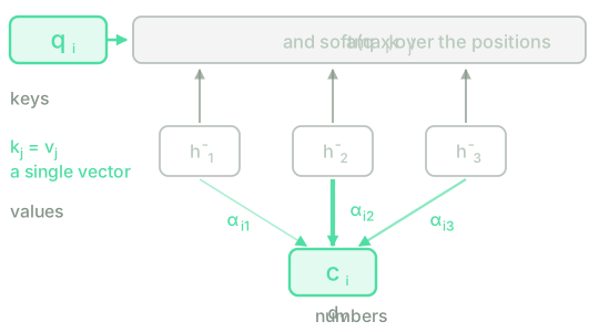
Each source position supplies two things with one vector: the key it is compared with and the value that gets mixed. No equation in the block asks for them to be the same.

The key and the value are the same vector, and no equation asks for it

Tying the two roles to one vector has a price: it forces the $d_h$ coordinates of $\bar{\mathbf{h}}_j$ to serve both purposes at once, to be good for being compared and good for being read.

The gradient's bookkeeping shows it better than the formula does. Untied, each role appears in a single place, so the chain rule follows a single route for each, summing over the $T_y$ steps because both lists are used in all of them:

\nabla_{\mathbf{v}_j}\ell = \sum_{i=1}^{T_y} \alpha_{ij}\,\nabla_{\mathbf{c}_i}\ell, \qquad \nabla_{\mathbf{k}_j}\ell = \sum_{i=1}^{T_y} \frac{\partial \ell}{\partial e_{ij}}\,\nabla_{\mathbf{k}_j} e_{ij},

and the step through the softmax is the one from the lesson on additive attentionBlock 4 · Lesson 4Bahdanau's attention (additive)The empty slot from the previous lesson, the function that scores a pair of states, gets filled with a tiny network: two projections that are added, a tanh that squashes the sum, and a vector that reads it out. You'll see why the tanh isn't decoration (without it the alignment stops depending on the step and freezes again), follow the gradient back to the encoder states, which it reaches along two routes (as a value and as something scored), and arrive at a derivative saying that a score is corrected only when its state differs from the mixture its row has already built., with one difference: it now says precisely what is compared with what:

\frac{\partial \ell}{\partial e_{ij}} = \alpha_{ij}\left(\nabla_{\mathbf{c}_i}\ell\right)^{\top}\left(\mathbf{v}_j - \mathbf{c}_i\right).

What gets compared with the mixture is that position's value; what receives the correction is its key. With one vector playing both roles, that sentence couldn't even be written.

And tying them back together gives the two-route formula again

Setting $\mathbf{k}_j = \mathbf{v}_j = \bar{\mathbf{h}}_j$ isn't a new case for the gradient: it's a shared weight, like the $\mathbf{W}_{hh}$ that runs across every position in the previous block's recurrence, or the $\mathbf{W}_a$ that scores every pair. An object that appears in two places receives the sum of what reaches it through each, so the two routes above add up:

\nabla_{\bar{\mathbf{h}}_j}\ell = \sum_{i=1}^{T_y} \alpha_{ij}\,\nabla_{\mathbf{c}_i}\ell + \sum_{i=1}^{T_y} \frac{\partial \ell}{\partial e_{ij}}\,\nabla_{\bar{\mathbf{h}}_j} e_{ij},

which is, term by term, the two-route line from the lesson on additive attentionBlock 4 · Lesson 4Bahdanau's attention (additive)The empty slot from the previous lesson, the function that scores a pair of states, gets filled with a tiny network: two projections that are added, a tanh that squashes the sum, and a vector that reads it out. You'll see why the tanh isn't decoration (without it the alignment stops depending on the step and freezes again), follow the gradient back to the encoder states, which it reaches along two routes (as a value and as something scored), and arrive at a derivative saying that a score is corrected only when its state differs from the mixture its row has already built.. There, the second term was expanded for the additive score as $\mathbf{W}_{ha}^{\top}\nabla_{\mathbf{p}_{ij}}\ell$ , which is this same term with $\nabla_{\bar{\mathbf{h}}_j} e_{ij}$ written out. What looked like a quirk of the architecture in that lesson (the gradient reaches this state along two routes) turns out to be a consequence of having tied two roles together.

The whole grid with three matrices

Stack the three roles by rows, as the previous lesson stacked the states: $\mathbf{Q} \in \mathbb{R}^{T_y \times d_k}$ with step $i$ 's query in row $i$ , and $\mathbf{K} \in \mathbb{R}^{T_x \times d_k}$ and $\mathbf{V} \in \mathbb{R}^{T_x \times d_v}$ with position $j$ 's key and value in row $j$ of each (transposed, because in this course vectors are columns). With the score in its cheapest form, the dot product, the three operations above fit in one line:

\text{Attention}\left(\mathbf{Q}, \mathbf{K}, \mathbf{V}\right) = \text{softmax}\left(\mathbf{Q}\mathbf{K}^{\top}\right)\mathbf{V} \in \mathbb{R}^{T_y \times d_v},

with the softmax taken by rows, so that each row of $\mathbf{Q}\mathbf{K}^{\top}$ (one query against the $T_x$ keys) comes out summing to $1$ . The function's name is the one the paper that fixed this form gave it, and it's how you'll find it written everywhere.

Now for the question that decides the next block: where has $\mathbf{W}_a$ gone? The previous lesson's grid was $\mathbf{S}\mathbf{W}_a\bar{\mathbf{H}}^{\top}$ , so group the first two factors and compare with the line above. Out come $\mathbf{Q} = \mathbf{S}\mathbf{W}_a$ (that is, $\mathbf{q}_i = \mathbf{W}_a^{\top}\mathbf{s}_{i-1}$ ) and $\mathbf{K} = \mathbf{V} = \bar{\mathbf{H}}$ . The matrix hasn't disappeared: it has stopped being part of the comparison and become part of what is compared. And with it out of the way, the function $a$ is left as the bare dot product for good. Everything a model wants to learn about how to compare has to be built into how $\mathbf{Q}$ and $\mathbf{K}$ are made, a matter this line is silent about and the next block is almost entirely about.

The additive score can't be moved like that, and the argument is the one from the lesson on additive attentionBlock 4 · Lesson 4Bahdanau's attention (additive)The empty slot from the previous lesson, the function that scores a pair of states, gets filled with a tiny network: two projections that are added, a tanh that squashes the sum, and a vector that reads it out. You'll see why the tanh isn't decoration (without it the alignment stops depending on the step and freezes again), follow the gradient back to the encoder states, which it reaches along two routes (as a value and as something scored), and arrive at a derivative saying that a score is corrected only when its state differs from the mixture its row has already built.: between the two projections and the read-out there's a $\tanh$ , and a non-linear function of a sum doesn't split among its terms. So this three-matrix form, the one the next block inherits, exists thanks to the choice the previous lesson made, not in spite of it.

One debt is left, and it's worth stating out loud because you're going to see it written. The next block's form carries one more factor:

\text{Attention}\left(\mathbf{Q}, \mathbf{K}, \mathbf{V}\right) = \text{softmax}\!\left(\frac{\mathbf{Q}\mathbf{K}^{\top}}{\sqrt{d_k}}\right)\mathbf{V}.

That divisor answers what the previous lesson measured without fixing: with freshly initialised weights, the largest weight in one row reached $0.851$ against the $0.167$ of an even share, because an unbounded dot product grows with the size of the vectors it multiplies. In this notation that size has a name, $d_k$ , which is why the fix fits in a single division. Where the root comes from (and why $\sqrt{d_k}$ and not something else) is the subject of a lesson in the next block, on the scaled dot-productComing up · Block 5 · Lesson 3 · In SpanishLa raíz que faltaba en la atenciónDe la fórmula de la atención queda un solo símbolo sin justificar, y no se justifica midiendo: se cuenta. Una puntuación es una suma de d_k términos, y lo que crece al añadir sumandos no es su tamaño sino cuánto se aleja del cero la suma, que va con la raíz de d_k. Lo que ese tamaño le hace al softmax es lo que el curso ya vio dos veces con otra ropa: la fila se cierra sobre una posición, las dos derivadas del softmax se apagan a la vez y las dos únicas matrices que hay antes de las puntuaciones dejan de recibir gradiente. Dividir entre la raíz devuelve las puntuaciones a una escala que no menciona la anchura del modelo, y con ellas el reparto y el gradiente.; for now, all you need is to know that the factor is there and which problem it answers.

The three arguments, in NumPy

The whole function is two lines, and what the cell checks is that nothing changed when the names did. First it recovers the previous lesson's grid by handing out the roles (the query is the decoder state rewritten by $\mathbf{W}_a$ , and the key and the value are the same encoder state). Then it unties them: one projection to compare with, $d_k = 3$ coordinates wide, and another to mix, $d_v = 7$ wide. Pay particular attention to the last three lines.

import numpy as np

T_y, T_x, d_h = 8, 6, 5
rng = np.random.default_rng(4)
S = rng.normal(size=(T_y, d_h)) * 0.6      # row i: the decoder state s_{i-1}
H = rng.normal(size=(T_x, d_h)) * 0.6      # row j: the encoder state at position j
Wa = rng.normal(size=(d_h, d_h)) * 0.4     # the multiplicative score's matrix


def softmax_rows(E):
  Z = np.exp(E - E.max(axis=1, keepdims=True))
  return Z / Z.sum(axis=1, keepdims=True)


def attention(Q, K, V):
  A = softmax_rows(Q @ K.T)               # (T_q, T_k): one weight per pair, rows that sum to 1
  return A @ V, A                         # (T_q, d_v): one mixture of values per query


# 1. The previous lesson, with the roles handed out: the query is the decoder state
#    rewritten by Wa, and the key and the value are the same encoder state.
Y, A = attention(S @ Wa, H, H)
print("same grid as the previous lesson:", bool(np.allclose(A, softmax_rows(S @ Wa @ H.T))))
print("every row of A sums to 1:", bool(np.allclose(A.sum(axis=1), 1.0)))
print("shapes:  Q", (S @ Wa).shape, " K", H.shape, " V", H.shape, " ->  output", Y.shape)
print()

# 2. Untied: two different projections of the same state, not even the same width.
d_k, d_v = 3, 7
Wq, Wk, Wv = (rng.normal(size=(d_h, d_k)), rng.normal(size=(d_h, d_k)), rng.normal(size=(d_h, d_v)))
Q, K, V = S @ Wq, H @ Wk, H @ Wv
Y2, A2 = attention(Q, K, V)
print("with d_k =", d_k, "and d_v =", d_v, " ->  A", A2.shape, " output", Y2.shape,
    " rows that sum to 1:", bool(np.allclose(A2.sum(axis=1), 1.0)))

# 3. Role against role: which one sets the weights and which one reaches the decoder.
other_K, other_V = rng.normal(size=(T_x, d_k)), rng.normal(size=(T_x, d_v))
print("changing V moves the map:   ", bool(not np.allclose(attention(Q, K, other_V)[1], A2)))
print("changing K moves the map:   ", bool(not np.allclose(attention(Q, other_K, V)[1], A2)))
print("changing V moves the output:", bool(not np.allclose(attention(Q, K, other_V)[0], Y2)))

numpy

The first run downloads the Python interpreter (~15 MB). After that it stays in the browser cache and is reused across every lesson.

Replacing the values wholesale doesn't move a single weight of the map, while replacing the keys moves all of it. That's the separation the last three lessons couldn't show, because there was one vector and touching it changed both things at once. Look at the shapes in the second part too: the query is $3$ wide, the output is $7$ wide, and the map is still $8 \times 6$ , one row per step and one column per position. Change d_v to $2$ and run it again: the output shrinks and the map doesn't flinch.

Test your intuition

Five questions: who plays each role in what you already know, how big the output is, what happens when you touch only the values, how the gradient reaches each role, and where $\mathbf{W}_a$ ended up.

In the attention of the last three lessons, which vector plays each role?

The query is the decoder state

\mathbf{s}_{i-1}

, and the key and the value are one and the same vector: the encoder state

\bar{\mathbf{h}}_j

, one per source position.The query is the context

\mathbf{c}_i

, the key is

\mathbf{s}_{i-1}

and the value is

\bar{\mathbf{h}}_j

.The query is

\mathbf{s}_{i-1}

, the key is

\bar{\mathbf{h}}_j

and the value is the vector of the token at that source position.The query is

\mathbf{s}_{i-1}

, the key is

\mathbf{W}_a

(what the decoder state is compared against) and the value is

\bar{\mathbf{h}}_j

An attention call with $T_x = 12$ pairs, queries and keys of $d_k = 64$ coordinates, and values of $d_v = 32$ . How many numbers does one query return?

numbers

A margin of ±0 is accepted.

You swap the values $\mathbf{v}_j$ for others and leave the queries and the keys as they were. What happens to the weight map $\mathbf{A}$ ?

It doesn't move. The values don't enter the score, so every weight stays the same down to the last decimal place; only the output changes, since it's the mixture of those values.It changes completely: the weights measure how much each position contributes, and that has to be computed from what is going to be mixed.It changes only if the new values are a different width, because then the softmax normalises over an axis of a different size.Neither the map nor the output moves: as long as the weights sum to

1

, the mixture returns the same thing.

With the key and the value untied (two different vectors at each position), tick everything that's true about how the gradient of the loss reaches them.

Select every correct option. This is graded all-or-nothing: there is no partial credit.

A single route reaches

\mathbf{v}_j

, the one through the mixture, and it sums over the steps:

\sum_i \alpha_{ij}\nabla_{\mathbf{c}_i}\ell

.A single route reaches

\mathbf{k}_j

, the one through the score, and it passes entirely through

\partial\ell/\partial e_{ij}

.If the two roles are tied back into one vector, that vector receives the sum of the two routes, which is the formula from the lesson on additive attentionBlock 4 · Lesson 4Bahdanau's attention (additive)The empty slot from the previous lesson, the function that scores a pair of states, gets filled with a tiny network: two projections that are added, a tanh that squashes the sum, and a vector that reads it out. You'll see why the tanh isn't decoration (without it the alignment stops depending on the step and freezes again), follow the gradient back to the encoder states, which it reaches along two routes (as a value and as something scored), and arrive at a derivative saying that a score is corrected only when its state differs from the mixture its row has already built..Once they're untied, the derivative with respect to a score stops comparing anything: without one vector playing both roles, the subtraction that appeared in it can't be written.

Where does the previous lesson's matrix $\mathbf{W}_a$ end up when the grid is written as $\mathbf{Q}\mathbf{K}^{\top}$ ?

Inside the queries. With

\mathbf{q}_i = \mathbf{W}_a^{\top}\mathbf{s}_{i-1}

(that is,

\mathbf{Q} = \mathbf{S}\mathbf{W}_a

) and the keys equal to the encoder states,

\mathbf{Q}\mathbf{K}^{\top}

is the previous lesson's grid without a figure changed, and the score is left as the bare dot product.It got lost along the way:

\mathbf{Q}\mathbf{K}^{\top}

has no parameters, so the three-matrix form only works for the parameter-free variant.It's inside the softmax, which applies it to each row before normalising it.It's in the values,

\mathbf{V} = \bar{\mathbf{H}}\mathbf{W}_a

, which is where the parameters fit without disturbing the weights.

Write attention(Q, K, V), this lesson's function. It takes the queries Q, of shape $(T_q, d_k)$ with one row per query, the keys K, of shape $(T_k, d_k)$ , and the values V, of shape $(T_k, d_v)$ : one key and one value per position. It returns the pair (output, A), in that order: the output, of shape $(T_q, d_v)$ , and the weight map $\mathbf{A}$ , of shape $(T_q, T_k)$ , already normalised by rows.

The score is the dot product of each query with each key, with no matrix in between. Write it with matrix products, without looping over the pairs, and don't write into the arrays you receive.

The first run downloads the Python interpreter (~15 MB); after that it stays in the browser cache. This challenge is much easier to solve on a physical keyboard: on a phone, read it and come back later.

With the names in place, what's missing looks different. $\mathbf{K}$ and $\mathbf{V}$ exist in full as soon as the encoder finishes reading: they depend only on the source, and none of their rows waits for any other. $\mathbf{Q}$ is different. Its rows are made one at a time, because each query is a decoder state and each decoder state needs the previous step's context. Two of the three matrices are complete in one go while the third still moves in single file, which is the previous lesson's outstanding debt, told in this lesson's vocabulary.

And that's where the course turns. The first lesson of the next block, on removing the recurrence, takes the one remaining question seriously: if what strangles the parallelism is the recurrence, and attention already knows how to read a whole sequence without walking through it step by step, what's left once you take the recurrence out? The answer fills the rest of the course, and you reach it with the three words and the three letters already in place, which is the one thing this block had to accomplish.

Was this helpful?