Luong's attention (multiplicative)

A model with attention scores pairs: one number for each output step and each input position, and those numbers become the weights that mix the encoder states. The previous lesson, on Bahdanau's additive attention, filled the slot that computes them with a small network (a hidden layer of $d_a$ units and a linear read-out, trained along with everything else), and it left one cost standing: scoring a pair means building a whole vector of $d_a$ coordinates only to reduce it to the single number that was wanted.

This lesson asks whether it takes a hidden layer to say that two vectors correspond. Linear algebra has been producing that number since Block 1 with no network in between, and in 2015 Luong, Pham and Manning proposed using it with a single adjustment. What comes out doesn't look like a network; it looks like a product. And since the two forms are comparable in quality (the experiments in their papers measure that; no derivation does), what decides between them is everything else: what they cost, how much memory they move, and what shape their computation takes.

Go back to what the score has to do. A number that goes up when two vectors point the same way has been in the course since the lesson on the bag of wordsBlock 1 · Lesson 5Bag of words and TF-IDFSumming the one-hot vectors of a document gives a count vector where the function words rule. Weighting each coordinate by how rare the entry is in the rest of the corpus fixes that, and the logarithm that does it is no trick: it comes from measuring information.: the dot product $\mathbf{u}^{\top}\mathbf{v}$, whose normalised version is cosine similarity. It would be a free score (zero parameters) and a function of the pair, which is the condition the previous lesson declared non-negotiable: $\mathbf{s}_{i-1}^{\top}\bar{\mathbf{h}}_j$ can't be split into one opinion about a state plus another about the other.

What fails is a hidden assumption. The dot product multiplies coordinate against coordinate, so it takes for granted that coordinate $k$ of the decoder means the same thing as coordinate $k$ of the encoder, on the same scale. But these are two different recurrences, with two sets of weights and two jobs (one reads Spanish, the other writes English), and nothing forces them to have chosen the same directions for the same things, or even to have the same number of coordinates. So the fix is to change basis first and measure afterwards.

Multiplying instead of adding

The multiplicative score puts a matrix between the two states and does nothing else:

with $\mathbf{W}_a \in \mathbb{R}^{d_h \times d_h}$. Read it from right to left: $\mathbf{W}_a\bar{\mathbf{h}}_j$ is the encoder state rewritten in the decoder's coordinates, and the dot product with $\mathbf{s}_{i-1}$ then measures what a dot product always measures. There's no hidden layer, no saturation and no space of the function's own, so the previous lesson's $d_a$ drops out of the problem.

Count the weights: $d_h^2$, and as before, none of them depends on the pair or on the lengths. With $d_h = 64$ that's $4\,096$, against the $4\,128$ the additive score needed with $d_a = 32$. Practically the same, which is useful to know early: what separates the two scores isn't how many weights they have, but what they do with them.

This is the place to say what the course leaves out. Luong, Pham and Manning also change where the context comes in (they score with the current step's state, $\mathbf{s}_i$, and mix in the context after the recurrence instead of inside it), and this course doesn't follow them. It keeps the placement from the lesson on the idea of attentionBlock 4 · Lesson 3The idea of attention: looking backThe encoder computes one state per token, and the architecture uses only one of them. Handing them all to the decoder runs into a problem of shape (there are as many states as tokens, but the decoder has a fixed size), and the way out is to mix them: each output step gets a context vector of its own, a weighted sum of every state, with weights that add up to one and change from step to step. This lesson defines that mixture, shows that the fixed summary of the previous two lessons is the same mixture with its weights frozen, and explains where the weights come from (a score for each pair, normalised with a softmax over the input positions) without yet saying what computes the score., so that across that lesson, the previous one and this one, only one thing changes. The comparison is of the function $a$, with everything else held fixed.

The gradient is shorter than the additive score's, for the same reason the computation is. The three derivatives of a score come from differentiating a product of three factors:

None of them carries a factor $1 - \tanh^{2}$, because there's no $\tanh$ to differentiate. And everything above $e_{ij}$ in the chain is the previous lesson's, without a comma changed: the step through the softmax and the derivative

never mentioned what form $a$ had. The attention stays as it is; only the alignment model changes.

Without a matrix: the dot product

The extreme case is to take $\mathbf{W}_a$ equal to the identity, which leaves the score as

and the function $a$ without a single parameter to train. What it asks in return is exactly what the matrix was there to avoid asking: that the two sides be the same width ($d_h$ coordinates in both) and that they have also learned to use those coordinates in the same way. That's a lot to demand when the encoder and the decoder are two different networks, each trained for its own language, which is why the matrix is the form Luong's paper takes as its default. The parameter-free variant stays in the course (it's the cheapest way to score that exists), but it only holds up where the two sides share a basis.

The whole grid in one matrix product

So far the lesson has written the scores one at a time. Now stack them. Store the encoder states by rows in $\bar{\mathbf{H}} \in \mathbb{R}^{T_x \times d_h}$ (row $j$ is $\bar{\mathbf{h}}_j^{\top}$, transposed because in this course vectors are columns) and the decoder's in $\mathbf{S} \in \mathbb{R}^{T_y \times d_h}$, whose row $i$ is $\mathbf{s}_{i-1}^{\top}$, the state that scores step $i$. Then the $T_x \cdot T_y$ scores are a single object:

with the softmax applied by rows, that is, over the input positions, as in the lesson on the idea of attentionBlock 4 · Lesson 3The idea of attention: looking backThe encoder computes one state per token, and the architecture uses only one of them. Handing them all to the decoder runs into a problem of shape (there are as many states as tokens, but the decoder has a fixed size), and the way out is to mix them: each output step gets a context vector of its own, a weighted sum of every state, with weights that add up to one and change from step to step. This lesson defines that mixture, shows that the fixed summary of the previous two lessons is the same mixture with its weights frozen, and explains where the weights come from (a score for each pair, normalised with a softmax over the input positions) without yet saying what computes the score.. Check entry $(i, j)$: row $i$ of $\mathbf{S}\mathbf{W}_a$ is $\mathbf{s}_{i-1}^{\top}\mathbf{W}_a$ and column $j$ of $\bar{\mathbf{H}}^{\top}$ is $\bar{\mathbf{h}}_j$, so their product is $e_{ij}$ and nothing else.

The additive score can't be written this way, and no amount of cleverness changes that. Its two projections do come out, but the $\tanh$ sits between the sum and the read-out, so a three-dimensional block (one entry per pair, and $d_a$ coordinates within each) has to be materialised before it can be reduced to numbers.

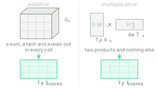
The counts put a price on that difference. Take $T_x = T_y = 60$ and $d_h = d_a = 256$, a long sentence and a small model. In products and sums the two are close: about $8.8$ million for the additive score against about $4.9$ million for the multiplicative one, a factor of less than two, and in both most of the work goes into the projections. Where they part ways is everything else. The additive score evaluates the $\tanh$ $921\,600$ times and the multiplicative one never does. Above all, the additive score has to store those $921\,600$ numbers ($7.4$ MB for each pair of sentences, before multiplying by the batch size), while the multiplicative one needs only the $3\,600$ scores and the $60$ states already projected. Between the two, the factor is exactly $d_a$: one number per pair against $d_a$ numbers per pair.

There's also a difference of shape that doesn't show up in any of those numbers. The multiplicative score's work is two matrix products; the additive score's is sums and $\tanh$ over a three-dimensional block, coordinate by coordinate. The same amount of arithmetic, organised in those two ways, doesn't cost the same on the hardware that trains these networks, which is built precisely for the first (that's what the lesson on the forward passBlock 2 · Lesson 4The forward pass in matrix formA whole layer collapses into one matrix product, and a whole batch fits into that same product with one row per example. That is where the transpose comes from (examples stack as rows, but an example itself is a column), and chaining those products from input to output gives you the forward pass, whose parameter cost never depends on how many examples go through at once. measured, with a loop against a product).

What's left is the honest part, and it's what opens the next block. Writing $\mathbf{S}$ means having all $T_y$ decoder states, and the decoder is recurrent: $\mathbf{s}_{i-1}$ needs $\mathbf{c}_{i-1}$, which needs row $i-1$ of $\mathbf{A}$, which needs $\mathbf{s}_{i-2}$. While the model translates, the grid fills up row by row and the big product never gets to happen. What can come out of the loop is $\mathbf{W}_a\bar{\mathbf{H}}^{\top}$, which depends only on the source and needs computing once per sentence, leaving each decoder step a single matrix-vector product:

row $i$ of unnormalised scores. The score is no longer the computation's bottleneck. What strangles the parallelism now is the recurrence that produces the states.

The two scores, in NumPy

The first cell computes the multiplicative alignment the short way and checks that the product says nothing different from scoring the pairs one by one. Look at the last two lines too: with $\mathbf{W}_a$ equal to the identity, the score reduces to the dot product of the two states.

The line that matters is the loop's: scoring pair by pair gives the same numbers as the product, which is all there is to check about the short form. The largest-weight line holds a surprise. With freshly initialised weights the map already shares out unevenly (one row takes $0.851$ when an even share would be $0.167$), which didn't happen in the previous lesson at a similar size, where the largest weight in each row hovered around the even share. The difference is the $\tanh$: it bounds each coordinate before $\mathbf{v}_a$ reads it, so the additive score starts out small. The multiplicative score has nothing to bound it, and its size grows with the size of the states. That peak isn't an alignment, it's the direction $\mathbf{W}_a$ happened to take at random; what the formula guarantees isn't that it starts out saying something, but that there's a route along which to train it. Scores that grow without bound as the model gets larger are a real problem, and the next block brings a one-line fix.

Everything above the last line is the previous section told in code: the arithmetic is similar, but the $\tanh$ and the $7.4$ MB of intermediates aren't. The last line depends on the machine and the browser, and it still tells you something, because the difference it measures isn't small: the multiplicative score takes around an order of magnitude less time, and the exact factor changes from run to run without ever getting close to one. There's an experiment that settles the question. Change $d_a$ to $64$ and run the cell again: the additive score now does less arithmetic than the multiplicative one ($2.2$ million operations against $4.9$) and still takes longer, about twice as long in the runs behind this lesson. What the clock is measuring isn't how many operations there are.

Test your intuition

Four questions: what the matrix adds, how many weights the score carries, what the additive score stores that the other doesn't, and whether the grid can be computed in one go.

With the two scores side by side, something shows that neither could reveal alone. In both, the encoder state enters the mechanism twice, through different doors: once as an argument of $a$, which is where its weight is decided, and once as a term of $\mathbf{c}_i$, which is how its content reaches the decoder. The decoder state, by contrast, enters only once, always from the same side: it's the one asking. That makes three roles, and neither formula requires the first two to be played by the same vector. One vector plays both only because nobody has yet proposed separating them.

Separating them and giving them names (query, key and value) is the job of the next lesson, the last in the block, and it's the most important one in this course. It doesn't change a single equation you've already seen: it rewrites the same ones in the words and symbols Block 5 writes everything in, including the choice of score this lesson has now justified. Nor does the change of names fix what was left pending here (the states still arriving one at a time); that's work for the next block, and it pays to arrive there with the names already in place.