The chain rule, in earnest

Of the three prerequisites this course starts from, one is the chain rule, and up to now the course has differentiated using the version everyone learns first: two one-variable functions chained, their two derivatives multiplied. That version produced both calculations this block has needed so far, the correction of the output layer and the gradient of a lone neuron. The previous lesson, on gradient descent, left training solved except for one piece: the step knows exactly what to do with the gradient, but for a network with hidden layers there is still no way to actually compute one. This lesson is that missing piece, and it turns out to be pure calculus.

Look closely at where things actually get complicated, because it is not where it seems. Take the review network with three answers instead of two (positive, negative and neutral, the classes the lesson on loss functionsBlock 2 · Lesson 5Loss functions: MSE and cross-entropyA loss sums up in one number how badly the network is doing, and between two candidates its derivative is what decides. Mean squared error hands over its smallest correction exactly where the network is wrong with the most confidence; cross-entropy, which comes from reading the output as a probability, leaves that derivative at the plain difference between what was predicted and the label. used to arrive at the softmax): eight inputs, four hidden neurons, three outputs. Pick any weight in the first layer, say the one the first hidden neuron gives fun, and nudge it by a thousandth. Its neuron's value changes: so far, the usual calculation. What comes next is not usual at all, because that neuron feeds all three output neurons, all three feed into the loss, and all three have now moved. One number touched, three effects rippling out through different routes and meeting back up at the end. The one-variable rule has nowhere to put that.

What needs counting is not the neurons, it is the paths running from a weight all the way to the loss.

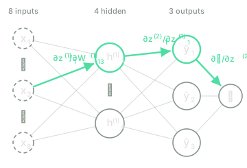
Of the three plausible answers (keep the heaviest path, average them, or add them all up), only one is actually right, and it is worth understanding why before you use it.

When one variable arrives by several paths

Set the network aside for a moment. Let $\mathcal{L}$ be a function of $m$ variables $u_1, \dots, u_m$, and let each of them, in turn, be a function of one and the same variable $t$. Then $\mathcal{L}$ depends on $t$ even without ever mentioning it, and its derivative is

one summand per intermediate variable. Each summand has the shape of the familiar rule (how much $\mathcal{L}$ responds to $u_k$, times how much $u_k$ responds to $t$), and what's new is that there are $m$ of them, and that they add. Within a path you multiply; across paths you add.

That sum is not a convention, and where it actually comes from is the one thing in this lesson that isn't bookkeeping. $\mathcal{L}$ being differentiable at a point means that, close to it, the function looks like a linear function of the displacements $\Delta u_1, \dots, \Delta u_m$, and a linear function of $m$ numbers is a sum of $m$ terms, one per number. The paths aren't competing with each other: each contributes its own share, and the shares add because the approximation they come from was already a sum to begin with.

Now bring that back to the network. The weight you were moving, the one the first hidden neuron gives fun, is $\mathbf{W}^{(1)}_{13}$ (row $1$, that neuron's; column $3$, that vocabulary entry's), and the intermediate variables are the three pre-activations of the output layer, $z^{(2)}_1$, $z^{(2)}_2$ and $z^{(2)}_3$. There are two more links along the way, so each summand carries four factors:

None of these four is new. The first is the result the lesson on loss functionsBlock 2 · Lesson 5Loss functions: MSE and cross-entropyA loss sums up in one number how badly the network is doing, and between two candidates its derivative is what decides. Mean squared error hands over its smallest correction exactly where the network is wrong with the most confidence; cross-entropy, which comes from reading the output as a probability, leaves that derivative at the plain difference between what was predicted and the label. closed the output layer with, by pairing softmax and cross-entropy together. The second comes from $z^{(2)}_k$ being a sum in which $h^{(1)}_1$ appears exactly once, multiplied by its weight. The third is the derivative of the activation, tabulated for all three candidates back in the lesson on activation functions and non-linearityBlock 2 · Lesson 2Activation functions and non-linearityThe step passes along the sign of the pre-activation and drops everything else, and its derivative is zero wherever it even exists. Sigmoid, hyperbolic tangent and ReLU keep the magnitude instead and have a real derivative; none of them can be a straight line, because chaining affine functions together only ever gives back another affine function.. And the fourth belongs to the previous lesson: the pre-activation is linear in its weights, so the derivative with respect to any one of them is the input that multiplies it. The only genuinely new fact was that the three paths add.

The object that replaces the derivative

That formula handles one weight. The network has $51$, and fifty-one separate sums full of indices are not really an answer, this needs to go up a level.

Let $\mathbf{u} : \mathbb{R}^{n} \to \mathbb{R}^{m}$. Its derivative at a point is the Jacobian, the matrix that gathers every partial derivative of every output with respect to every input,

with one row per output coordinate and one column per input coordinate. That ordering, output first, belongs to the whole course, and from it fall out the two things this block does with a Jacobian.

The first is that composing turns back into multiplying. If $\mathbf{x} \in \mathbb{R}^{n}$ produces $\mathbf{u} \in \mathbb{R}^{m}$ and this in turn produces $\mathbf{v} \in \mathbb{R}^{p}$, then

a product of a $p \times m$ matrix by an $m \times n$ one that delivers exactly the $p \times n$ matrix you need. The dimension that gets summed over and disappears is $m$, the intermediate variables, exactly the way the width shared by two layers disappeared in the forward passBlock 2 · Lesson 4The forward pass in matrix formA whole layer collapses into one matrix product, and a whole batch fits into that same product with one row per example. That is where the transpose comes from (examples stack as rows, but an example itself is a column), and chaining those products from input to output gives you the forward pass, whose parameter cost never depends on how many examples go through at once..

And that product isn't some new object, it's the previous one stacked up. Expand entry $(i, j)$ using the definition of the matrix product:

which is exactly the sum over paths from the previous section, written for output $i$ and input $j$: the $m$ routes from $x_j$ to $v_i$, one per intermediate variable you could pass through. The sum over paths and the matrix product are the same calculation, and the computer performs the second one without anyone ever writing an index.

The loss is a scalar, and that is where the transpose comes from

The second thing comes from looking at the far end of the chain. $\mathcal{L}$ returns a single number, so in its case $m = 1$ and its Jacobian is a one-row matrix, $\partial\mathcal{L}/\partial\mathbf{x} \in \mathbb{R}^{1 \times n}$. The gradients in this course are columns, like every vector in it, so one is the transpose of the other, $\nabla_{\mathbf{x}}\mathcal{L} = \left(\partial\mathcal{L}/\partial\mathbf{x}\right)^{\top}$. Transpose the composition above (remembering that transposing a product reverses the order of its factors):

an $n \times m$ matrix times a vector of $m$ coordinates, which returns exactly the vector of $n$ you wanted. That's the shape of everything left in this block: a gradient comes in on the right, leaves converted into the gradient of the previous layer, and the transposed Jacobian is what performs that conversion.

Hold on to one observation this lesson doesn't actually use. A chain of Jacobians can be evaluated either by multiplying the matrices among themselves first, or by carrying the output's gradient backwards through one transpose after another. Both give the same answer, since the matrix product is associative, but they don't cost the same: the first multiplies matrices by matrices, and the second only ever multiplies matrices by vectors.

A coordinate-wise activation has a diagonal Jacobian

One concrete Jacobian is still missing, the activation's, and it comes out far cheaper than its size would suggest. With $\mathbf{h} = \varphi(\mathbf{z})$ applied coordinate by coordinate, each output looks at exactly one input: $h_i$ depends on $z_i$ and on nothing else, so $\partial h_i / \partial z_j = 0$ the moment $i \neq j$. Of the whole $m \times m$ matrix, only the diagonal survives:

where $\text{diag}(\mathbf{v})$ is the square matrix carrying $\mathbf{v}$ on its diagonal and zeros everywhere else. Multiplying by it amounts to multiplying coordinate by coordinate, which has its own symbol, the Hadamard product:

From here on, nobody actually builds the matrix: it's $m$ products instead of $m^{2}$, and $m$ numbers stored instead of $m^{2}$, of which $m^{2} - m$ would be zeros anyway. With ReLU (rectified linear unit), the diagonal is $0$ or $1$ and acts as a mask: a hidden neuron with a negative pre-activation gets a zero in its entry, and that zero cuts off every path running through it. This is the dying ReLU from the lesson on activation functionsBlock 2 · Lesson 2Activation functions and non-linearityThe step passes along the sign of the pre-activation and drops everything else, and its derivative is zero wherever it even exists. Sigmoid, hyperbolic tangent and ReLU keep the magnitude instead and have a real derivative; none of them can be a straight line, because chaining affine functions together only ever gives back another affine function., seen from the other side.

Softmax is the exception, and it's worth flagging: it mixes every coordinate together, so its Jacobian has not a single zero anywhere in it. It isn't needed here, because the lesson on loss functionsBlock 2 · Lesson 5Loss functions: MSE and cross-entropyA loss sums up in one number how badly the network is doing, and between two candidates its derivative is what decides. Mean squared error hands over its smallest correction exactly where the network is wrong with the most confidence; cross-entropy, which comes from reading the output as a probability, leaves that derivative at the plain difference between what was predicted and the label. already differentiated it together with cross-entropy, and out of that pairing came $\hat{\mathbf{y}} - \mathbf{y}$, the gradient this whole chain starts from.

One weight, three paths and three ways of measuring them

The cell feeds the review the movie is fun and i recommend it into the network of eight inputs, four hidden neurons and three outputs, and computes $\partial\mathcal{L}/\partial\mathbf{W}^{(1)}_{13}$ (the same weight as in the previous section) three different ways: a numerical probe, the sum of the three paths, and the product of the Jacobians. I set the weights by hand, so you'll see these exact numbers and no others. Run it, compare the three figures, and then look at the fourth.

Go back to the previous section's formula, but with the four factors stacked into their proper objects: the summation sign disappears inside the matrix product.

The diagonal is written out in full here (not as the previous section's cheap Hadamard product) because the goal is to show the Jacobian exactly as it is, not to save on arithmetic; $\mathbf{e}_1 \in \mathbb{R}^{4}$ is $1$ at hidden neuron $1$ and $0$ at the other three, the only one that $\mathbf{W}^{(1)}_{13}$ actually moves. What does save effort is the order: evaluated left to right (row times matrix, three times over), nothing larger than a row of four numbers ever appears, which is the observation from the transpose section put into practice. That's step 3 of the cell below.

All three agree at $-0.09208080$, and the probe is the one with the least right to: it knows nothing about the network's structure at all, it only evaluates the loss with the weight nudged a hundred-thousandth up and a hundred-thousandth down. That it matches the chain result exactly is the check worth keeping handy for whenever a hand-written derivative refuses to add up.

The fourth figure is the one that teaches what this lesson is really about. Forgetting a path (the third one, through the output neuron for the neutral class) leaves the derivative at $-0.16541038$, almost double what it should be. And look closely at the three summands, because the error isn't one of size: the first two are negative and the third is positive. That path was pulling the other way, so removing it doesn't trim the correction down, it inflates it instead. A forgotten path doesn't give you an approximate derivative, it gives you the derivative of an entirely different function.

The last line prints the shapes in the chain, $(1, 3) \times (3, 4) \times (4, 4) \times (4, 1)$. And in the $\varphi^{\prime}$ row there's a zero: the fourth hidden neuron has its pre-activation at $-1.5$, it's switched off for this particular review, and its entry on the diagonal cuts off whatever tried to pass through it.

Test your intuition

Four questions (a sum of paths worked out by hand, why they add, the shapes of a Jacobian, and the order of the product), plus a challenge that is the entire chain rule.

Everything needed to differentiate any network is now on the table, and laid out like this it's useless in practice. The cell computed the derivative of one weight, and to get it, it walked the entire chain: the error at the output layer, the second layer's matrix, the diagonal of the activation. The very next weight needs that same walk repeated, with only a single different factor at the end, and so do the other forty-nine weights in this network. With a vocabulary of twenty thousand entries and a hundred and twenty-eight hidden neurons, that's upwards of two and a half million walks, identical except for the last step, and not even the fastest computer in the world has time to spare for that.

The waste becomes obvious the moment you name it: those walks share almost everything, and whatever is shared gets recomputed once per parameter anyway. What's actually needed is to reverse the direction of travel: compute once, starting from the last layer, how much the loss owes every pre-activation in the network, and let each weight read its derivative off a quantity that's already sitting there. That procedure has a name of its own, gets derived layer by layer with every index in view, and is the next lesson, on backpropagation.