Gradient descent

The training question can now be written out in full, and writing it doesn't solve it. The previous lesson, on loss functions, put the last piece in place: a rule that compares what the network answers with what it should have answered, and sums it all up in one number. Searching for the parameters that make that number smallest is now a well-posed question, and there's still no way to answer it by trial and error. The network from the lesson on the forward passBlock 2 · Lesson 4The forward pass in matrix formA whole layer collapses into one matrix product, and a whole batch fits into that same product with one row per example. That is where the transpose comes from (examples stack as rows, but an example itself is a column), and chaining those products from input to output gives you the forward pass, whose parameter cost never depends on how many examples go through at once. holds $41$ numbers; with a vocabulary of twenty thousand entries and a hidden layer of $128$ neurons, that becomes $2\,560\,257$, and every single one of them is a real number.

There is, though, a much smaller question that does get answered. Take one of those $41$ parameters on its own, raise it by a hundredth, leave the other $40$ untouched, and evaluate the loss again: if it went up, that parameter was moving the wrong way; if it went down, the right one. It's a local answer (it doesn't say where the minimum is, only which way the ground slopes from here), and, taken to the limit, it's had a name since the seventeenth century: the partial derivative of the loss with respect to that parameter. Probing all $41$ costs $41$ evaluations. Differentiating gives you all of them without probing a single one, and for one neuron the whole count fits on a line; getting the same result with hidden layers in the way takes up the rest of this block.

Before differentiating anything, look at the terrain itself. Fix every one of a network's parameters but two, and the loss becomes a function of those two numbers, which draws as a surface full of valleys and hillsides. The one in the explorable below comes from no real network at all: I made it up so it fits on a plane and has two bottoms instead of one.

The descent never compares the two valleys, because it can't see them. From wherever it stands, it has access to exactly one thing (how much the loss changes when you move a little in each direction), and that's all it uses to decide the next step. Right on the ridge, that slope points nowhere useful: the derivative is zero without the spot being a bottom, a saddle point, and there the descent stays put instead of moving any further down.

The gradient points uphill, and that is why it is subtracted

Call $\theta$ all of the network's parameters at once (the weights and biases of every layer, stacked into a single vector of $P$ coordinates), and $\mathcal{L}(\theta)$ the loss over the batch. The gradient is the vector that gathers one partial derivative per parameter, $\nabla_{\theta}\mathcal{L} \in \mathbb{R}^{P}$. Each of its coordinates says how fast the loss changes when one parameter moves and the rest hold still: exactly what the hundredth-step probe measured, only exact this time, and without ever evaluating anything twice. For the neuron from the lesson on the artificial neuronBlock 2 · Lesson 1The artificial neuronA weighted sum and a threshold are all a single unit needs to turn a vector into a decision. Its weights sit perpendicular to a boundary that splits the space in two, and the number it computes before deciding measures how far the input has landed from that boundary., with its weights $\mathbf{w} \in \mathbb{R}^{d}$ and its bias $b$, that's $d + 1$ numbers:

The first thing worth noticing is that $\nabla_{\theta}\mathcal{L}$ has the exact same shape as $\theta$. That's no accident: it's precisely what lets you subtract one from the other.

What's left is to justify why you subtract that particular vector and nothing else. Take any direction, a vector $\mathbf{u} \in \mathbb{R}^{P}$ of length $1$, and ask how much the loss changes as you move a little in it. That's the directional derivative, which for a function with partial derivatives turns out to be a dot product,

and it's bounded. The Cauchy-Schwarz inequality gives

with equality only when $\mathbf{u}$ is parallel to the gradient. Of every possible direction, then, the gradient's own direction raises the loss the most, and the opposite one lowers it the most. No other direction lowers it more per unit of step.

From there, the whole rule follows. Starting from some initial parameters $\theta_0$, each step subtracts the scaled gradient:

where the subscript counts steps ($\theta_5$ is the parameters after five steps, not the fifth coordinate of anything), and $\eta > 0$ is the learning rate, the one number in the whole formula that you actually choose. That's gradient descent, in its entirety.

That repeating this actually lowers the loss shows up in the first-order approximation. Near $\theta_t$, the loss looks much like its own tangent plane,

and the descent step is precisely $\Delta = -\eta\,\nabla_{\theta}\mathcal{L}$, so

What gets subtracted is a squared norm, and so it's never negative: as long as the gradient isn't zero, the step goes down. The entire catch sits in that equation's sign, an $\approx$: the equality belongs to the tangent plane, not to the loss itself, and it only holds "nearby". How near is exactly what $\eta$ decides.

One concession worth saying out loud: this lesson's batch is all ten reviews at once, so every step looks at every example before moving anything. That's called batch gradient descent, and it's far from the only way to fix $B$. At the other extreme, stochastic gradient descent (SGD) sets $B = 1$: each step looks at a single example and costs almost nothing, but the gradient it uses is no longer the exact one from this lesson, it's a noisy estimate of it, computed from one example instead of ten. The mini-batch sits in between, with $B$ somewhere between those two extremes (a few tens or hundreds of examples, typically), and it's the option that wins out in practice. It's not only that a set of millions won't fit in memory at once: even when it would fit whole, many cheap, somewhat noisy steps tend to train faster in wall-clock time than a few exact, expensive ones. The size of the dataset pushes towards the mini-batch, but that's not the only reason to choose it, and the full batch isn't only a matter of small datasets either: it's used here because there are ten examples and it makes the arithmetic easier to follow by hand, not because ten marks any real boundary.

And letting $B$ vary brings in a word that until now was unnecessary: an epoch is one complete pass through all $N$ training examples. With $B = N$, which is this lesson's case, a step and an epoch are the same thing (each step already runs through the whole set), which is why "step" has been enough on its own so far. As soon as $B < N$, the two stop matching: it takes $N / B$ steps to complete one epoch, and training in earnest means repeating many epochs, not one.

A step too long raises the loss

To see what $\eta$ actually does, it helps to use a loss whose sum can be worked out in closed form, so take the smallest one there is: a single parameter, $\mathcal{L}(w) = w^{2}$, with the minimum at $w = 0$ and $\dfrac{d\mathcal{L}}{dw} = 2w$. The rule becomes

a multiplication by the same constant at every step. Iterating from $w_0$,

and a power tends to zero exactly when its base is smaller than $1$ in absolute value. The full condition is $\lvert 1 - 2\eta \rvert < 1$, that is, $0 < \eta < 1$, and the factor itself tells you what happens in each stretch:

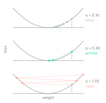
That particular $1$ in the limit belongs to this parabola and not to every one of them. With $\mathcal{L}(w) = a\,w^{2}$, the derivative becomes $2aw$, the factor becomes $1 - 2\eta a$, and the condition becomes $\eta < 1/a$: the more sharply the loss curves, the shorter the step has to be. The awkward part is that a real network curves differently in every direction, while $\eta$ stays a single number shared by all of them.

The explorable dives straight into that problem, $\mathcal{L} = x^{2} + 20y^{2}$: almost flat along $x$ and very steep along $y$. The count above, applied coordinate by coordinate, asks for $\eta < 1$ in the first direction and $\eta < 1/20 = 0.05$ in the second, and the second one wins.

With $\eta = 0.05$ (the value it starts at), the factor for the steep coordinate is exactly $-1$, and the trajectory does in two dimensions exactly what the fourth row of the table does in one: alternate without ever advancing. The first button's bowl is convex (a single bottom, so whoever descends ends up in the same place), and it survives the whole range of the slider: its steepest direction only demands $\eta < 1/3$. The fact that one step size can work for one direction and fail for another has fixes with their own names, momentum, Adam, and they lie outside this course.

With a single layer, the gradient comes out of a line

What's left is to bring the descent from $\theta$ down to a concrete parameter, and with the reviews' neuron the work is already half done. It's a neuron with a sigmoid on the output and cross-entropy as the loss, exactly the pair the previous lesson derived: for one example, $\partial \ell / \partial z = \hat{y} - y$. The only thing missing is how $z$ depends on each weight, and that comes straight from the neuron's own definition, $z = \mathbf{w}^{\top}\mathbf{x} + b = \sum_{j=1}^{d} w_j x_j + b$, where each $w_j$ appears exactly once, multiplied by $x_j$:

Chaining the two derivatives together,

which in vector form becomes

That formula is really saying two separate things, and they're worth pulling apart. The error $\hat{y} - y$ is a single number that multiplies every coordinate the same way: it fixes how much correction there is to go around. And $\mathbf{x}$ decides how that correction gets shared out: a vocabulary entry that never appears in the review has $x_j = 0$ and its weight doesn't budge a thousandth, while one that appears twice pulls twice as hard. The neuron only ever learns from what it has actually seen.

The batch loss is the mean of the $B$ per-example losses, so its gradient is the mean of the $B$ individual gradients:

where the second form writes the first as a single product: with $d_L = 1$ the predictions and labels are columns of $B$ numbers, $\mathbf{X}^{\top}$ has shape $d_0 \times B$, and the result is exactly the column of $d_0$ coordinates you need. The bias comes out of that same sum, minus the $\mathbf{x}_i$:

All of this cost only two derivatives, because $z$ depends on $\mathbf{w}$ directly: between a weight and the loss there sit a sum and a sigmoid, and nothing else.

Descent by hand, and a neuron that learns on its own

The first cell is the parabola from above, with no network and no NumPy involved: five steps from $w_0 = 1$ at the figure's three rates, alongside the closed form. Run it and compare the two blocks.

The three rows match the three curves in the figure. With $\eta = 0.10$, the factor is $0.8$ and five steps leave $w$ at $0.32768$: it moves in the right direction but slowly. With $0.40$, the factor is $0.2$ and within two steps $w$ is already $0.04$. With $1.05$, the factor is $-1.1$, the signs alternate, the magnitudes grow, and the final loss is $2.59$: two and a half times what it was at the start, after five steps that were supposed to lower it.

The second cell trains for real. The neuron is the same one from the lesson on the artificial neuronBlock 2 · Lesson 1The artificial neuronA weighted sum and a threshold are all a single unit needs to turn a vector into a decision. Its weights sit perpendicular to a boundary that splits the space in two, and the number it computes before deciding measures how far the input has landed from that boundary., with the same ten reviews and the same vocabulary, except this time its weights start at zero: with $\mathbf{w} = \mathbf{0}$ and $b = 0$, the sigmoid answers $0.5$ across all ten, the worst score among the three networks the previous lesson ranked. There isn't a single random number anywhere in this cell, so you'll see these exact values and no others. Run it and watch the loss fall.

The first line is the starting point: loss $0.6931$, which is $\log 2$, and five correct out of ten, the score of any network that gives the same answer to all ten reviews. Twenty-five steps later, the loss is down to $0.0913$ and the correct count has reached ten, and by step $200$ it's fallen all the way to $0.0131$. Compare that with the $0.2208$ from the eight weights I set by eyeballing the reviews: the descent overtakes my version before step $25$ and keeps improving from there. Nobody ever told the neuron what any word means.

The final weights confirm it. The largest, $+3.911$, goes to recommend, and the smallest, $-3.428$, to slow: entirely on its own, the descent has sorted the opinion words by sign. But look at the two that expose the limit of a set of only ten examples. movie ends at $-1.493$ and the at $-0.832$, and neither one says anything at all about a film. Both come out negative for the same reason, and it's a coincidence, not a meaning: movie shows up in four negative reviews and two positive ones, the in two negative and one positive, so across these ten they read as evidence against. The descent does exactly what it was asked to do, lower the loss over these ten reviews rather than over the language itself, and in doing so it hands movie a weight against the film heavier than some words carrying a real opinion ever get. With only ten examples, a neuron can't tell an opinion apart from a coincidence.

Test your intuition

Three questions: a descent worked out by hand, why the step heads in that particular direction, and what the method guarantees against what it doesn't.

The method is complete, and the neuron that has now finished learning has exactly one layer. That's not an incidental detail of the example, it's the very condition that made the last section possible: between a weight and the loss there are two steps, and two chained derivatives close out the count. Put a hidden layer in between, and the path branches. A weight in the first layer moves the output of its hidden neuron; that output feeds into every neuron of the next layer, and each one contributes to the loss in its own way. The descent's rule doesn't change by a single letter. What stops being available is the gradient itself, and without it there's nothing left to subtract.

The chain rule used twice already, the one-variable version, doesn't cover that case: it's written for a quantity that reaches the next one by a single path. How a composition gets differentiated when the intermediate variables are vectors, and what object replaces the derivative once there are many inputs and many outputs at once, is the next lesson, on the chain rule. Turning that into a procedure that walks an entire network without repeating a single computation takes up the rest of this block.