Why the MLP fails on sequences

23 min read

An input layer is exactly as wide as it was built to be; a text is however long it happens to be. The previous block, on the multilayer perceptron (MLP), kept bumping into that tension without ever quite naming it. Its review classifier got about $86.7\%$ of unseen reviews right, and what held it back wasn't the network but the input: the order of the tokens never made it through the door. Fixing that means changing the input, and changing the input means going back to $\mathbf{W}^{(1)}$ , which has had $d_0$ columns from the moment it was built.

The fix anyone would think of first is to line the tokens up in a row. Each one brings its own vector (the embedding from the lesson on dense representations), and gluing those vectors end to end writes the order into where each one sits: position becomes a coordinate, and there's no sum to wipe it out. The fix lasts until the second text. the cinematography is superb brings four vectors and weak script brings two, so they produce inputs of two different widths, and a layer that multiplies by $\mathbf{W}^{(1)}$ accepts exactly one.

There's a second consequence too, and it only shows up once you draw it.

At the top, a horizontal bar labelled x on its left, divided into six equal segments numbered one to six, one per position in the sequence. The third and fifth segments are shaded green, each with the label "not" above it. Below, a wide rectangle labelled W one, as wide as the bar and divided into six blocks of columns that line up with the segments above and are numbered the same way; only the third and fifth blocks are shaded. Two dotted green lines run down, one from the third segment to the third block and one from the fifth segment to the fifth block. Under the rectangle, its shape: d one by T max times d model. — The same vocabulary entry in two different positions never touches the same weights: in one case it's multiplied by the third block, in the other by the fifth, and those two blocks are adjusted separately.

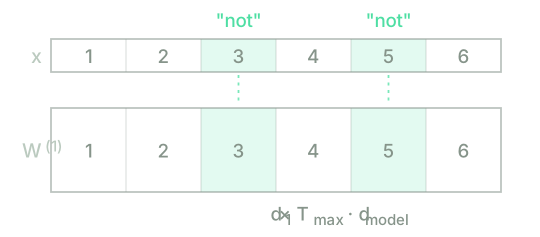
The rest of this lesson is that figure, first written out in symbols and then measured with NumPy.

A sequence that doesn't fit a fixed-size input

The tokeniser turns a document into a sequence of tokens $w_1, \dots, w_T$ . That length $T$ belongs to this particular document; the next one will have a different one. Each position contributes the vector of its vocabulary entry, $\mathbf{x}_t = \mathbf{e}_{w_t} \in \mathbb{R}^{d_{\text{model}}}$ , its own row of $\mathbf{E}$ . Stacking them all into a single column means writing

\mathbf{x} = \left[\mathbf{x}_1 ; \mathbf{x}_2 ; \dots ; \mathbf{x}_T\right] \in \mathbb{R}^{T \cdot d_{\text{model}}},

where the semicolons stack downwards: the result is one vector of $T \cdot d_{\text{model}}$ numbers, not a matrix with $T$ rows. The order is in there, intact, and reading it off is a matter of looking at the right stretch. The letter now appears in two forms on purpose, so it's worth pinning them down: $\mathbf{x}$ with no subscript is the input for the whole example, as it was throughout the previous block, and $\mathbf{x}_t$ is the piece that position $t$ contributes.

On the other side sits a layer that won't negotiate. $\mathbf{W}^{(1)} \in \mathbb{R}^{d_1 \times d_0}$ has $d_0$ columns, a number fixed when the network is built, which knows nothing about the document that's about to come in. With $\mathbf{x}$ of length $T \cdot d_{\text{model}}$ and $T$ changing from one text to the next, the product $\mathbf{W}^{(1)}\mathbf{x}$ is defined for documents of one length and undefined for every other. This isn't a matter of rounding or of training: the multiplication doesn't exist.

The only way out that leaves the architecture alone is to fix a number of positions, $T_{\max}$ , and force every document to that length:

\mathbf{x}_t = \begin{cases} \mathbf{e}_{w_t} & \text{if } t \leq T,\\ \mathbf{0} & \text{if } T < t \leq T_{\max}, \end{cases}

keeping only the first $T_{\max}$ positions when $T > T_{\max}$ . Filling the leftover positions with the zero vector is called padding; cutting at $T_{\max}$ is truncation. With both in place, $d_0 = T_{\max} \cdot d_{\text{model}}$ for every document, and the network can be built.

Each half of that arrangement has its own cost, and both deserve spelling out. Truncation throws away the whole tail of any long document, and it does so by position. That's nothing like the out-of-vocabulary (OOV) problem from the lesson on the vocabulary, where the casualties were the rare types, which is why so little was lost. Here the most frequent entry in the corpus can be the one that goes, if it happens to sit at position $T_{\max} + 1$ . Padding pays at the other end: with $T_{\max}$ set to reach the longest document, a document of average length enters the network with more than half its vector at zero.

Each position learns on its own

Now slice $\mathbf{W}^{(1)}$ along the same seams as the input. Its $d_0 = T_{\max} \cdot d_{\text{model}}$ columns fall into $T_{\max}$ consecutive blocks of $d_{\text{model}}$ columns each, $\mathbf{W}^{(1)} = \left[\mathbf{W}^{(1)}_1 \mid \dots \mid \mathbf{W}^{(1)}_{T_{\max}}\right]$ with $\mathbf{W}^{(1)}_t \in \mathbb{R}^{d_1 \times d_{\text{model}}}$ (here the subscript is a position in the sequence, not a coordinate), and the product splits the same way:

\mathbf{z}^{(1)} = \mathbf{W}^{(1)}\mathbf{x} + \mathbf{b}^{(1)} = \sum_{t=1}^{T_{\max}} \mathbf{W}^{(1)}_t\,\mathbf{x}_t + \mathbf{b}^{(1)}.

Nothing has actually changed yet: it's the same product as always, grouped into stretches instead of single columns. The interesting part shows up when you differentiate.

The lesson on backpropagationBlock 2 · Lesson 8Backpropagation: the full derivationDifferentiating weight by weight forces a run over the network once per parameter, and those runs share almost everything. Backpropagation instead computes a single number per pre-activation (that neuron's error), in one pass from the end back to the beginning, and lets each weight read its own derivative as the product of that error with whatever it had in front of it. boiled a layer's gradient down to one line, $\nabla_{\mathbf{W}^{(l)}}\ell = \boldsymbol{\delta}^{(l)}\left(\mathbf{h}^{(l-1)}\right)^{\top}$ , and for the first layer $\mathbf{h}^{(0)} = \mathbf{x}$ , so

\nabla_{\mathbf{W}^{(1)}}\ell = \boldsymbol{\delta}^{(1)}\,\mathbf{x}^{\top} \in \mathbb{R}^{d_1 \times d_0}.

That outer product splits by columns at exactly the places where $\mathbf{W}^{(1)}$ was split, and the piece that goes to each block is

\nabla_{\mathbf{W}^{(1)}_t}\ell = \boldsymbol{\delta}^{(1)}\,\mathbf{x}_t^{\top} \in \mathbb{R}^{d_1 \times d_{\text{model}}}.

The split by columns, step by step

The outer product is defined coordinate by coordinate: entry $(i, j)$ of $\boldsymbol{\delta}^{(1)}\mathbf{x}^{\top}$ is $\delta^{(1)}_i \cdot x_j$ , with $i$ running over the $d_1$ neurons and $j$ over the $d_0$ columns.

Column $j$ belongs to block $t$ when $(t-1) \cdot d_{\text{model}} < j \leq t \cdot d_{\text{model}}$ , and within that block it's column $j - (t-1) \cdot d_{\text{model}}$ . Since concatenation defines $x_j$ as coordinate $j - (t-1) \cdot d_{\text{model}}$ of $\mathbf{x}_t$ , the submatrix made of those $d_{\text{model}}$ columns holds $\delta^{(1)}_i \cdot x_{t,k}$ at entry $(i, k)$ , which, entry for entry, is $\boldsymbol{\delta}^{(1)}\mathbf{x}_t^{\top}$ .

The split works because the two things being split, the columns of $\mathbf{W}^{(1)}$ and the coordinates of $\mathbf{x}$ , are split at the same places. And nothing else enters the calculation: every block receives the whole of $\boldsymbol{\delta}^{(1)}$ , so the only thing that distinguishes one block's gradient from another's is which vector of the sequence it gets multiplied by.

Read that slowly, because it's the key result of the lesson. The gradient of block $t$ depends on $\mathbf{x}_t$ and on no other part of the input. If that position was padded, then $\mathbf{x}_t = \mathbf{0}$ and the block receives the zero matrix: that example teaches it nothing at all, not a little and not a lot. And if the input is one-hot, $\mathbf{x}_t = \mathbf{o}_{w_t}$ has a single one, so $\boldsymbol{\delta}^{(1)}\mathbf{o}_{w_t}^{\top}$ is zero everywhere except in one column: inside block $t$ , the only column that moves is the one for the vocabulary entry that sat in that position.

Put those two facts together and you get the claim this section is named after. The column that represents an entry inside block $t$ is adjusted only by the examples in which that entry appeared at position $t$ . If an entry never reached position 5 in the training set, the matching columns of block 5 stay exactly as initialisation left them, however many steps gradient descent takes; and whatever the network has worked out about that same entry at position 3 is stored in other weights, which position 5 can't reach.

What it costs in weights

$\mathbf{W}^{(1)}$ has shape $d_1 \times d_0$ , so it holds $d_1 \cdot d_0$ weights, and with a concatenated input that comes to

d_1 \cdot T_{\max} \cdot d_{\text{model}} \quad \text{weights}.

Plug in some ordinary sizes (embeddings of $d_{\text{model}} = 100$ , a hidden layer of $d_1 = 128$ neurons and $T_{\max} = 30$ positions) and the first layer alone has $384\,000$ weights. For comparison, the previous lesson's review classifier, a single hidden layer over a bag of words, had $5\,257$ parameters in total. Reading paragraphs instead of sentences, with $T_{\max} = 300$ , pushes the figure up to $3\,840\,000$ .

The growth itself isn't the problem; it's a symptom. The real issue underneath is that the $3\,456\,000$ weights added in going from $30$ positions to $300$ are new weights: they start from their initialisation and inherit nothing of what the first thirty blocks learned. Meanwhile the corpus still has the same examples it always had, so more positions means spreading those examples across more blocks: less experience per parameter, at exactly the moment there are more parameters to train.

Measuring it with NumPy

A small experiment puts numbers on all this. I made up the sequences for the course: six positions, eight vocabulary entries, and the label is $1$ whenever not appears among them. The catch is where it appears: in training, only in the first four positions; in the test, only in the last two. That's the only difference between the two sets.

The cell trains the same network twice on the same data: once on the concatenation of the six positions, and once on their bag of words, the same one-hot vectors summed into eight coordinates. The training loop is the one from the lesson on implementing an MLPBlock 2 · Lesson 9Implementing an MLP from scratchThe four pieces of training are all derived by now, and no cell has ever run them one after another. Assembling them costs stacking the backward pass by rows (bringing along the 1/B the mean introduces) and making the one decision no formula makes: where the weights start from. Start them all equal and they stay equal forever, which is exactly why initialisation has to be random., without a single line changed. Read the output in three parts: what concatenation does, what the bag of words does with the same data, and what has happened to each block of $\mathbf{W}^{(1)}$ .

import numpy as np

V = ["the", "film", "is", "very", "good", "long", "fun", "not"]
NOT, T = 7, 6                                 # "not" is the last entry; six positions
rng = np.random.default_rng(0)


def corpus(n, positions):
  S = rng.integers(0, NOT, size=(n, T))     # filler, drawn from the first seven
  y = np.zeros((n, 1))
  y[::2] = 1.0                              # exactly half carry "not"...
  for i in np.nonzero(y[:, 0])[0]:
      S[i, rng.choice(positions)] = NOT     # ...and only where they're told
  U = np.eye(len(V))[S]                     # (n, 6, 8): one one-hot per position
  return U.reshape(n, T * len(V)), U.sum(1), y   # concatenate them, or sum them


C_train, B_train, Y_train = corpus(600, [0, 1, 2, 3])   # "not" in positions 1-4
C_test, B_test, Y_test = corpus(300, [4, 5])            # in the test, only in 5-6


def train(X_train, X_test, steps=1500, eta=0.5, d1=16):
  r = np.random.default_rng(1)
  W1, b1 = r.normal(size=(d1, X_train.shape[1])) * 0.1, np.zeros(d1)
  W2, b2 = r.normal(size=(1, d1)) * 0.1, np.zeros(1)
  W1_init = W1.copy()

  def output(X):
      H = np.tanh(X @ W1.T + b1)
      return H, 1.0 / (1.0 + np.exp(-(H @ W2.T + b2)))

  def accuracy(X, Y):
      return float(((output(X)[1] >= 0.5) == (Y == 1.0)).mean())

  for _ in range(steps):                    # the previous block's loop, untouched
      H, P = output(X_train)
      D2 = P - Y_train
      D1 = (D2 @ W2) * (1.0 - H ** 2)
      W1 -= eta * (D1.T @ X_train) / len(X_train)
      b1 -= eta * D1.sum(0) / len(X_train)
      W2 -= eta * (D2.T @ H) / len(X_train)
      b2 -= eta * D2.sum(0) / len(X_train)
  return (accuracy(X_train, Y_train), accuracy(X_test, Y_test),
          W1 - W1_init, output(X_test)[1])


acc_train, acc_test, moved, P_test = train(C_train, C_test)
print("concatenation   training %.3f   test %.3f" % (acc_train, acc_test))
print("bag of words    training %.3f   test %.3f" % train(B_train, B_test)[:2])
print('mean ŷ of the 150 test examples carrying "not": %.4f' % P_test[Y_test == 1.0].mean())

print('\nhow far the "not" column has moved in each block:')
for t in range(T):
  print("   position %d:  %.6f" % (t + 1, np.linalg.norm(moved[:, t * len(V) + NOT])))

numpy

The first run downloads the Python interpreter (~15 MB). After that it stays in the browser cache and is reused across every lesson.

The first line is the failure: $1.000$ on what the network has seen, $0.500$ on what it hasn't. And that $0.500$ isn't a coin toss. It gets all hundred and fifty test sequences that don't contain not right, and all hundred and fifty that do contain it wrong, because as far as it can tell they're identical to the first lot. The third line shows how far this goes: the mean $\hat{y}$ over the hundred and fifty positives is $0.0014$ . The network isn't wavering between the two answers; it's certain, and wrong.

The second line is the awkward one. The bag of words (the very representation this block set out to replace, the one that can't tell one order from another) scores $1.000$ on the shifted test. Its advantage is precisely what concatenation lacks: it has one coordinate for not, which collects the occurrences from all six positions at once, so a weight adjusted on what happened at position 2 works as it stands when not turns up at position 5. Concatenation gained order and lost exactly that.

The last part of the output is the formula, verified. The not column has moved about $2.4$ units in blocks 1 to 4, and $0.000000$ in blocks 5 and 6 (genuinely zero, not something rounded down to it), because its share of the gradient $\boldsymbol{\delta}^{(1)}\mathbf{x}_t^{\top}$ was zero on all six hundred examples at every one of the fifteen hundred steps. Change the initialisation and the figure for the first four blocks changes; the last two still read zero, and test accuracy still reads $0.500$ .

Test your intuition

Four questions: how many weights concatenation needs, why the unseen position stays invisible, what padding and truncation cost, and what you can and can't conclude from the bag of words winning this test.

Take an MLP over a concatenated input with $T_{\max} = 40$ positions, embeddings of $d_{\text{model}} = 128$ and a hidden layer of $d_1 = 64$ neurons. How many weights does $\mathbf{W}^{(1)}$ hold?

A margin of ±0 is accepted.

The cell trains with not only in the first four positions and tests with not only in the last two. Test accuracy sits at $0.500$ , and no amount of extra steps, extra hidden neurons or tweaking of the learning rate budges it. Why?

Because

\nabla_{\mathbf{W}^{(1)}_t}\ell = \boldsymbol{\delta}^{(1)}\mathbf{x}_t^{\top}

is zero in the not column of blocks 5 and 6 for every training example, so those columns finish exactly where they started.Because 600 examples aren't enough for the 768 weights in the first layer, and the network runs out of data to pin them down.Because the hyperbolic tangent saturates on one-hot inputs, so the gradient dies out before it reaches the first layer.Because the test set is unbalanced, and half its examples carry the wrong label.

Tick everything that is true of an MLP whose input is the concatenation of $T_{\max}$ positions.

Select every correct option. This is graded all-or-nothing: there is no partial credit.

Padding a position with the zero vector makes the gradient of that position's block exactly zero on that example.Truncating at

T_{\max}

loses text based on where it sits, not on how rare it is, so the same type can vanish from one document and survive in another.Raising

T_{\max}

from

30

60

doubles the weights in the first layer, and doubles the examples each block learns from as well.Two documents with the same tokens in a different order produce the same input.

In the cell's experiment, the bag of words passes the shifted test and concatenation doesn't. Does that mean you can conclude the bag of words is the better representation of the two?

TrueFalse

The two things this lesson has measured are really one. The fixed length forces truncation and padding because the first layer has exactly one block per position and not one more; and what's learned at one position never reaches the others because each block is adjusted only by its own. Both come from putting the whole sequence in front of the network at once, as if it were a single point in $\mathbb{R}^{d_0}$ with a great many coordinates, and neither can be fixed from within that idea: not with more neurons, not with more steps, and certainly not with a larger $T_{\max}$ , which makes both worse.

What's needed is a network in which position 5 is multiplied by the same weights as position 3, so that adjusting them on one occurrence adjusts them for every position. That forces two things at once: reading the sequence one position at a time rather than all in one go, and keeping what has already been read somewhere else (because if the matrix is the same at every position, the order can't be stored in it). That's the next lesson, on the simplest recurrent neural network (RNN) there is: a single matrix applied $T$ times, a state passed from one step to the next, and an input that no longer has to be the same length for every document.

Was this helpful?