Loss functions: MSE and cross-entropy

30 min read

Measuring isn't answering, and answering is all the network knows how to do. The previous lesson, on the forward pass in matrix form, closed off one half of the route from $\mathbf{X}$ to $\hat{\mathbf{Y}}$ : a chain of products that crosses every layer without ever once asking whether what it hands back looks anything like what it should. The other half starts here, by fixing a rule that compares $\hat{\mathbf{Y}}$ with $\mathbf{Y}$ and sums up, in a single number, how badly the batch is doing. That rule is called a loss function, and it has to be chosen carefully.

Plenty of rules would technically work, and the choice among them carries real weight. Take fun and i recommend it, which speaks well of the movie: its label is $y = 1$ , and the network answers with a number between $0$ and $1$ that grows the more it leans towards that class. Suppose it hands back $0.002$ . It's wrong, since it should have landed right up against $1$ , and it's wrong with total confidence, since it couldn't have sat any closer to $0$ . This lesson compares two candidates, mean squared error and cross-entropy, and both agree the loss is high here; that's not where they part ways. What separates them is how much that loss changes when a weight moves, and on an example like this one, the first candidate, the one most people would reach for instinctively, barely reacts at all.

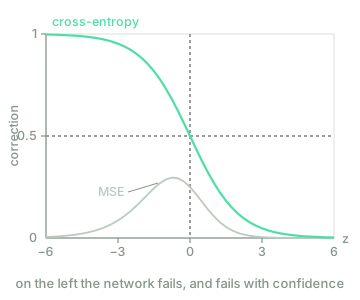
Before writing down a single formula, look at the shape of that difference. What's drawn below isn't the two losses themselves but the correction each one hands back: its derivative with respect to the pre-activation $z$ of the output neuron, which is exactly where the weights pull from (how much the loss shifts for every unit that $z$ moves). In green, cross-entropy; in grey, mean squared error (MSE). With the label at $1$ , the network gets it right towards the right of the drawing and gets it wrong towards the left.

A graph with the pre-activation z from minus 6 to 6 on the horizontal axis and the correction, from 0 to 1, on the vertical one. The cross-entropy curve, in green, enters through the top-left corner right up against 1, descends crossing the centre at 0.5 and ends right up against 0 on the right: it decreases without stopping. The MSE curve, in grey, enters through the bottom-left corner right up against 0, rises to a maximum of 0.30 shortly before the centre and falls back to 0 on the right: it is a hump with both tails on the floor. — The two tails of the MSE share the same value and mean opposite things: the one on the right is a network that gets it right and needs no correction, and the one on the left is a network that fails with confidence and still gets none. Cross-entropy only goes quiet at one end.

From predictions to a single number

The network hands over $\hat{\mathbf{Y}} \in \mathbb{R}^{B \times d_L}$ , and the examples bring their labels in an array of the same shape, $\mathbf{Y} \in \mathbb{R}^{B \times d_L}$ , row for row. A loss sums that pair up into one number, and it's built on two levels: a function $\ell$ that judges one example by comparing its prediction with its label, and the mean of the $B$ results that come out of it,

\mathcal{L} = \frac{1}{B} \sum_{i=1}^{B} \ell\left(\hat{\mathbf{y}}_i, \mathbf{y}_i\right),

where $\hat{\mathbf{y}}_i, \mathbf{y}_i \in \mathbb{R}^{d_L}$ are the prediction and the label of example $i$ : rows $i$ of $\hat{\mathbf{Y}}$ and of $\mathbf{Y}$ , written as columns. It's the mean rather than the sum precisely so $\mathcal{L}$ doesn't grow with $B$ . The two symbols share a name throughout the lesson (MSE, cross-entropy): $\ell$ and $\mathcal{L}$ are the same criterion, one per example and the other averaged over the whole batch.

Three demands fall on $\ell$ , and they don't carry equal weight: it has to return a number, it has to fall as the prediction approaches the label, and it has to have a derivative with respect to every parameter, because the method that corrects the weights runs entirely on those derivatives (the next lesson, on gradient descent). Almost anything satisfies the first two; the third is the one that actually rules candidates out, and it's the same criterion the lesson on activation functions and non-linearityBlock 2 · Lesson 2Activation functions and non-linearityThe step passes along the sign of the pre-activation and drops everything else, and its derivative is zero wherever it even exists. Sigmoid, hyperbolic tangent and ReLU keep the magnitude instead and have a real derivative; none of them can be a straight line, because chaining affine functions together only ever gives back another affine function. used to choose $\varphi$ : there, the step got ruled out for having a null derivative, not for measuring badly.

The first candidate measures the squared distance. Mean squared error is

\mathcal{L}_{\text{MSE}} = \frac{1}{B} \sum_{i=1}^{B} \left\lVert \hat{\mathbf{y}}_i - \mathbf{y}_i \right\rVert^{2}, \qquad \ell_{\text{MSE}}(\hat{y}, y) = (\hat{y} - y)^{2},

with the subscript naming which candidate it is, and the second form written for $d_L = 1$ , the review network, where $\hat{y}$ and $y$ are scalars: they've dropped the bold of $\hat{\mathbf{y}}_i$ and $\mathbf{y}_i$ , since with a single output the vector shrinks down to a single number. The square does two things at once: it strips away the sign, so overshooting and falling short cost the same, and it punishes large errors more than proportionally, since missing by $0.8$ costs sixteen times what missing by $0.2$ does, not four.

That's exactly the right criterion when the network is predicting a quantity: if the job is to guess how many stars its author gave the movie, the difference $\hat{y} - y$ is stars, and its square measures precisely what you want. Differentiating gives $\partial \ell_{\text{MSE}} / \partial \hat{y} = 2(\hat{y} - y)$ , the first good property of this loss: the correction stays proportional to the error. About that factor of $2$ , there's a convention I don't follow (many people put a $\tfrac{1}{2}$ in front so it cancels on differentiating), and it changes nothing measurable: multiplying every correction by a constant gets absorbed into the size of the step (how far the weights move on each update), which is what the next lesson adjusts.

Why it switches off exactly when it's most needed

Classifying isn't predicting a quantity, and there the arithmetic changes. The label is $0$ or $1$ , the output comes out of a sigmoid, $\hat{y} = \sigma(z)$ , and the derivative you actually need isn't the one with respect to $\hat{y}$ but the one with respect to $z$ , which is what the weights control. Chain the two, using $\sigma'(z) = \sigma(z)\left(1 - \sigma(z)\right)$ from the lesson on activation functionsBlock 2 · Lesson 2Activation functions and non-linearityThe step passes along the sign of the pre-activation and drops everything else, and its derivative is zero wherever it even exists. Sigmoid, hyperbolic tangent and ReLU keep the magnitude instead and have a real derivative; none of them can be a straight line, because chaining affine functions together only ever gives back another affine function.:

\frac{\partial \ell_{\text{MSE}}}{\partial z} = \frac{\partial \ell_{\text{MSE}}}{\partial \hat{y}} \cdot \frac{d\hat{y}}{dz} = 2\left(\hat{y} - y\right)\hat{y}\left(1 - \hat{y}\right).

Look at the product of the last two factors: it's the derivative of the sigmoid, and the lesson on activation functionsBlock 2 · Lesson 2Activation functions and non-linearityThe step passes along the sign of the pre-activation and drops everything else, and its derivative is zero wherever it even exists. Sigmoid, hyperbolic tangent and ReLU keep the magnitude instead and have a real derivative; none of them can be a straight line, because chaining affine functions together only ever gives back another affine function. already told you where that switches off: when $\hat{y}$ approaches $0$ or $1$ , that is, exactly when the network is sure of itself. The saturation that was a defect of the activation there resurfaces here, multiplying straight into the correction. With $y = 1$ and $z = -6$ (the network says no, confidently, and is wrong), the first factor is almost $-2$ , but $\hat{y}\left(1 - \hat{y}\right)$ is $0.0025$ , and the product stalls at $0.0049$ . The worst error in the whole batch gets the smallest correction in the whole batch.

This isn't some rare case picked by hand: it's the entire left half of the grey curve above. And no amount of adjusting the step size fixes a loss that confuses its own two tails, since it scales both of them the same way.

Cross-entropy, reading the output as a probability

The fix isn't to patch the formula, but to change what the network is supposed to be saying in the first place. Up to now $\hat{y}$ was a number between $0$ and $1$ ; read it instead as the probability the network assigns to the positive class, $\hat{y} = P(y = 1 \mid \mathbf{x})$ . With that reading, the probability it assigns to whichever label the example actually came with is written once, covering both cases,

P(y \mid \mathbf{x}) = \hat{y}^{\,y}\left(1 - \hat{y}\right)^{1-y},

because with $y = 1$ the second factor becomes $1$ and what's left is $\hat{y}$ , while with $y = 0$ it's the first factor that disappears. Assuming the $B$ examples are independent, the probability of observing the whole set is the product of all $B$ of them, and that quantity, viewed as a function of the parameters, is called the likelihood. It has to be made as large as possible. Multiplying $B$ numbers smaller than one drives the product towards zero very fast, so take logarithms instead (which preserve the order, so the maximum stays put), flip the sign so there's something to minimise, and divide by $B$ . Out comes cross-entropy:

\mathcal{L}_{\text{CE}} = -\frac{1}{B} \sum_{i=1}^{B} \left[\, y_i \log \hat{y}_i + \left(1 - y_i\right)\log\left(1 - \hat{y}_i\right) \right].

Read it example by example. One with $y_i = 1$ contributes $-\log \hat{y}_i$ : it's $0$ if the network gives it probability $1$ , and it grows without a ceiling as that probability falls towards zero; one with $y_i = 0$ looks at $1 - \hat{y}_i$ instead. That missing ceiling is the underlying difference from MSE, which never climbed above $1$ .

Now for the derivative, which is what actually decides things. Start from the loss of a single example,

\ell_{\text{CE}} = -y\log\hat{y} - (1-y)\log(1-\hat{y}),

differentiate it with respect to $\hat{y}$ , put the two terms over a common denominator, and chain with the sigmoid:

\begin{aligned} \frac{\partial \ell_{\text{CE}}}{\partial \hat{y}} &= -\frac{y}{\hat{y}} + \frac{1 - y}{1 - \hat{y}} = \frac{-y\left(1 - \hat{y}\right) + \hat{y}\left(1 - y\right)}{\hat{y}\left(1 - \hat{y}\right)} = \frac{\hat{y} - y}{\hat{y}\left(1 - \hat{y}\right)}, \\[4pt] \frac{\partial \ell_{\text{CE}}}{\partial z} &= \frac{\partial \ell_{\text{CE}}}{\partial \hat{y}} \cdot \frac{d\hat{y}}{dz} = \frac{\hat{y} - y}{\hat{y}\left(1 - \hat{y}\right)} \cdot \hat{y}\left(1 - \hat{y}\right) = \hat{y} - y. \end{aligned}

On the first line, the numerator simplifies because the two $y\hat{y}$ terms cancel out. On the second, the denominator turns out to be exactly the $\hat{y}(1 - \hat{y})$ the sigmoid contributes when you chain, and the two cancel each other away.

The correction turns out to be nothing but the plain difference between what the network said and what it should have said. On the example from before, that's $-0.9975$ instead of MSE's $0.0049$ . The saturation hasn't gone anywhere, the sigmoid still has it; what happens is that the loss's derivative carries the exact inverse factor that undoes it, which is why the final formula never even mentions $\varphi$ .

That's why it's called a loss and not an error: mean squared error genuinely measures something in the units of the label, while cross-entropy measures nothing of the kind (it's a logarithm of a probability), and it's still the better of the two. What decides isn't what they measure, but what they hand back once you differentiate them.

More than two classes: softmax

With three answers instead of two (positive, negative and neutral), the output layer has $d_L = 3$ neurons, and the sigmoid stops being any use: it squashes each coordinate on its own, and three numbers in $(0,1)$ don't automatically form a distribution. The function that does is softmax, the same one from the lesson on Word2Vec, which shared probability out among the entries of the vocabulary:

\hat{y}_k = \frac{e^{z_k}}{\sum_{m=1}^{d_L} e^{z_m}}, \qquad k = 1, \dots, d_L,

positive because it's an exponential, and summing to $1$ thanks to the denominator. The label is written one-hot, $\mathbf{y} \in \{0,1\}^{d_L}$ with a single $1$ at the position of the correct class $c$ , exactly the way the lesson on one-hot encoding encoded a vocabulary entry. The loss is the same one as before, written out for $d_L$ classes:

\ell = -\sum_{k=1}^{d_L} y_k \log \hat{y}_k = -\log \hat{y}_c,

where the second equality comes from the one-hot encoding cancelling every term but one. Only the probability the network gave the true class actually counts, though what it shares out among the others still matters, since the denominator ties all of them together.

The derivative, with the two kinds of index that have to be told apart

Differentiate $\ell = -\log \hat{y}_c$ with respect to each $z_j$ . The softmax mixes every coordinate into each one (moving $z_j$ moves the denominator, and with it all $d_L$ probabilities), so you need two separate computations, depending on whether $j$ is the correct class or not. Call $S = \sum_{m} e^{z_m}$ , with $\partial S / \partial z_j = e^{z_j}$ .

When $j = c$ , the numerator depends on $z_j$ too, and it's the derivative of a quotient:

\frac{\partial \hat{y}_c}{\partial z_c} = \frac{e^{z_c} S - e^{z_c} e^{z_c}}{S^{2}} = \frac{e^{z_c}}{S}\left(1 - \frac{e^{z_c}}{S}\right) = \hat{y}_c\left(1 - \hat{y}_c\right).

When $j \neq c$ , the numerator $e^{z_c}$ doesn't depend on $z_j$ at all, and only the denominator moves:

\frac{\partial \hat{y}_c}{\partial z_j} = e^{z_c} \cdot \left(-\frac{1}{S^{2}}\right) e^{z_j} = -\frac{e^{z_c}}{S}\cdot\frac{e^{z_j}}{S} = -\hat{y}_c\,\hat{y}_j.

With $\partial \ell / \partial \hat{y}_c = -1/\hat{y}_c$ , the chain rule gives both cases:

\frac{\partial \ell}{\partial z_c} = -\frac{1}{\hat{y}_c}\,\hat{y}_c\left(1 - \hat{y}_c\right) = \hat{y}_c - 1, \qquad \frac{\partial \ell}{\partial z_j} = -\frac{1}{\hat{y}_c}\left(-\hat{y}_c\,\hat{y}_j\right) = \hat{y}_j \quad (j \neq c),

and the two turn out to be the same expression, since $y_c = 1$ and $y_j = 0$ . Coordinate by coordinate:

\nabla_{\mathbf{z}}\,\ell = \hat{\mathbf{y}} - \mathbf{y}.

With $d_L = 2$ this reproduces the binary case exactly: the short formula from the previous section was never an accident of having a single output.

Both derivations land in the same place, and that's exactly why they're worth doing once: from here through the lesson on backpropagationComing up · Block 2 · Lesson 8Backpropagation: the full derivationDifferentiating weight by weight forces a run over the network once per parameter, and those runs share almost everything. Backpropagation instead computes a single number per pre-activation (that neuron's error), in one pass from the end back to the beginning, and lets each weight read its own derivative as the product of that error with whatever it had in front of it., the output layer never gets differentiated again, it goes in as $\hat{\mathbf{y}} - \mathbf{y}$ and that's the end of it. Softmax matters here because the rest of the course predicts over entire vocabularies, where the classes number in the tens of thousands.

The two losses over the ten reviews

The cell evaluates both candidates over the usual ten reviews, using the pre-activations of the neuron with hand-set weights from the lesson on the artificial neuron. Nothing here is random. Run it and look at three things: what order each column puts the networks in, where each correction switches off, and what happens with a logarithm of zero.

import numpy as np

# --- The usual ten reviews, with their labels and their pre-activations.
y = np.array([1., 0., 1., 0., 1., 0., 0., 1., 0., 1.])
z = np.array([2., -2., 2., -2., 2., -1., -2., 1., 0., 2.])
sigmoid = lambda z: 1.0 / (1.0 + np.exp(-z))


def mse(y_hat, y):
  return float(np.mean((y_hat - y) ** 2))


def cross_entropy(y_hat, y):
  p = np.clip(y_hat, 1e-12, 1.0 - 1e-12)          # without this, one 0 takes the whole mean with it
  return float(-np.mean(y * np.log(p) + (1.0 - y) * np.log(1.0 - p)))


# 1. Three networks: the hand-set-weight one, the same without conviction, and one that answers 0.5 to everything.
confident = sigmoid(z)
lukewarm = 0.5 + (confident - 0.5) * 0.1

print("%-25s %8s %8s %8s" % ("", "correct", "MSE", "CE"))
for name, p in [("hand-set-weight neuron", confident),
              ("the same, no conviction", lukewarm),
              ("answers 0.5 to everything", np.full(10, 0.5))]:
  correct = int(((p >= 0.5) == (y == 1.0)).sum())
  print("%-25s %8d %8.4f %8.4f" % (name, correct, mse(p, y), cross_entropy(p, y)))
print()

# 2. The correction of each loss, for an example whose label is 1.
print("%6s %6s %11s %11s %9s" % ("z", "ŷ", "|dMSE/dz|", "|dCE/dz|", "ratio"))
for zz in [-6.0, -3.0, 0.0, 3.0, 6.0]:
  s = sigmoid(zz)
  d_mse = abs(2.0 * (s - 1.0) * s * (1.0 - s))
  d_ce = abs(s - 1.0)
  print("%6.1f %6.3f %11.6f %11.6f %9.1f" % (zz, s, d_mse, d_ce, d_ce / d_mse))
print()

# 3. The logarithm of zero, and what covering it up costs.
p = np.array([0.9, 0.0, 0.5])
clipped = np.clip(p, 1e-12, 1.0)
with np.errstate(divide="ignore"):
  print("without clipping:", -np.log(p), " mean:", float(-np.mean(np.log(p))))
print("clipping:        ", np.round(-np.log(clipped), 2),
    " mean:", round(float(-np.mean(np.log(clipped))), 2))

numpy

The first run downloads the Python interpreter (~15 MB). After that it stays in the browser cache and is reused across every lesson.

The first table makes the case for the whole lesson. The count of correct answers ties the first two networks at nine out of ten: it can't tell apart saying $0.881$ from saying $0.538$ , because both land on the same side. The two losses separate them cleanly ( $0.049$ against $0.220$ for the confident network, $0.220$ against $0.633$ for the lukewarm one), and both put the one that answers $0.5$ to everything in last place, at $0.250$ and $0.693$ , which is $\log 2$ . They rank the networks the same way. What they don't do the same way is correct them.

That's the second table. At $z = -6$ , with the label at $1$ , cross-entropy hands back $0.9975$ and MSE hands back $0.0049$ : a ratio of $202.7$ . At $z = 0$ , with the network holding no opinion either way, the ratio drops to $2$ . The advantage grows towards the extremes, and one of those extremes is exactly where the network is wrong. The last row repeats that same $202.7$ with the network getting it right, and there both corrections are tiny, which is exactly as it should be.

The third experiment shows the detail that breaks a real implementation. $-\log 0$ is infinite, and one example the network assigns probability zero to is enough to send the mean of the entire batch to infinity and stop it from saying anything useful at all. Clipping at $10^{-12}$ avoids that, at a cost worth naming out loud: nobody ever actually measured that $27.63$ .

Test your intuition

Four questions (a cross-entropy worked out by hand, MSE when classifying, the clean correction, and the maximum of the softmax), plus a challenge on the output layer.

A network with a sigmoid on its output assigns $\hat{y} = 0.2$ to a review whose label is $y = 1$ . What is the cross-entropy of that example?

A margin of ±0.01 is accepted.

What happens to mean squared error when the output of the network is a sigmoid and the label is $0$ or $1$ ?

Its derivative with respect to

z

drags along the factor

\hat{y}(1 - \hat{y})

, which approaches zero exactly when the network is wrong with the most confidence: the worst error produces the smallest correction.It can give a number greater than

1

, and a bounded loss is essential for comparing different networks.It does not tell apart being wrong by a little from being wrong completely, because it squares, and the square erases that difference.It only works with two classes: with three or more it is no longer defined, and that is why cross-entropy is needed.

Tick everything that is true about this lesson's result $\dfrac{\partial \ell}{\partial z} = \hat{y} - y$ .

Select every correct option. This is graded all-or-nothing: there is no partial credit.

It comes from the

\hat{y}(1 - \hat{y})

that differentiating the sigmoid contributes being exactly the one that sat in the denominator from differentiating the logarithm, and the two cancel.With softmax and several classes it holds coordinate by coordinate: the correction of the output layer is

\hat{\mathbf{y}} - \mathbf{y}

.Its magnitude never reaches

1

, but it gets as close as it needs to as the network is wrong with more confidence.Since the formula does not mention

\varphi

, the sigmoid of the output layer can be removed without the correction changing.

softmax(z) and softmax(z + 100) return exactly the same thing. Why, and what is gained by subtracting the maximum of each row before exponentiating?

Because adding a constant multiplies numerator and denominator by the same

e^{100}

, which cancels. Subtracting the maximum uses that freedom so that the largest exponent is

e^{0} = 1

, so that nothing overflows and the result does not change.Because the softmax normalises at the end, and any shift is lost in that normalisation even though the numerators do change in relative value.Because subtracting the maximum is what makes the outputs sum to

1

; without that step the denominator is not enough to normalise them.Because the shift changes the result by less than

10^{-12}

, and at that scale the two values are indistinguishable in floating point.

Write the output layer of a network with several classes, over a whole batch and without Python loops:

softmax(Z) receives Z of shape $(B,\, d_L)$ and returns the probabilities row by row. Each row has to sum to $1$ , and the function has to survive large pre-activations: np.exp(1000) overflows.
cross_entropy(Y_hat, Y) returns the mean over the batch of $-\sum_k y_k \log \hat{y}_k$ , with Y encoded one-hot. A $\hat{y}_k$ equal to zero cannot return inf.

Neither function may write into the arrays it receives.

The first run downloads the Python interpreter (~15 MB); after that it stays in the browser cache. This challenge is much easier to solve on a physical keyboard: on a phone, read it and come back later.

There's now a number that says how badly the network is doing, and across this entire lesson, not a single weight has moved. All three networks arrived with their numbers already fixed, the loss has ranked them, which is all it was ever asked to do, and none of them has improved one bit for having been measured.

Training means making that number small, and the only thing you can actually touch to get there is the weights: changing them changes $\hat{\mathbf{Y}}$ , and through it, $\mathcal{L}$ . Of that movement, the derivative gives you the direction (if $\hat{y} - y$ is positive, raising $z$ raises the loss, so it needs to come down instead), but it doesn't give you the distance: it describes the slope right where you're standing and stops holding the moment you move. So the weights don't get corrected in one single leap, but in a series of steps, and the size of each step is itself a decision: too short and you never arrive, too long and you overshoot. How that size gets chosen, what goes wrong when it's chosen badly, and why repeating the process ends up finding the minimum without ever actually seeing it, is the next lesson, on gradient descent.

Was this helpful?