LSTM: gated memory

The previous lesson, on the vanishing gradient, closed with a diagnosis and a direction. The diagnosis: as long as every step of the backward pass goes through the same matrix, the result is a power of the distance. The direction: a state that moves forward as a running sum, and the network built around one, the long short-term memory (LSTM). But naming it isn't building it. A memory that only adds has a defect as serious as the one it fixes: it never erases anything. What's left is the hard part, deciding step by step what to keep, what to write over it, and how much of what's stored to let out.

An ordinary sentence shows that these are three decisions, not one. Take The cameras that the mayor installed in the square last year are broken. To write are rather than is, the network has to carry the plural of cameras across ten positions, without mayor or square (both singular, both closer) overwriting it along the way. Carrying it intact is one thing; storing it when cameras appears, and not at every passing word, is another; and keeping it stored through those ten positions without letting it drive the network's answers at the positions in between is a third. The vanilla recurrent neural network (RNN) handles all three with the same move, because it only has one: rewriting the whole of $\mathbf{h}_t$ at every step. That's why it can't do any of them well.

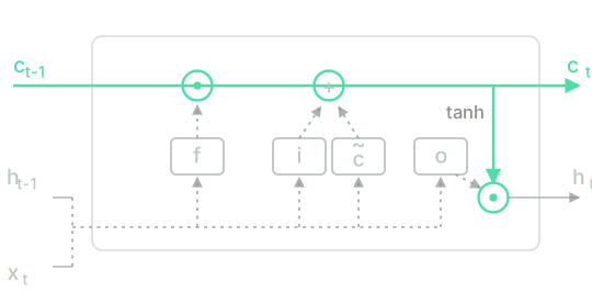
Separating the three jobs starts with separating two states. Alongside the $\mathbf{h}_t$ you already know, a second vector appears, the cell state $\mathbf{c}_t \in \mathbb{R}^{d_h}$, which is the memory proper, and the way it moves forward is the only genuinely new idea in this lesson. Everything else in the LSTM exists to control that vector.

Three gates, each fixing a failure of the previous version

Start from the additive path on its own and add what it's missing as we go. The candidate is the vector that step $t$ proposes to store, computed by an ordinary layer from the token and the previous state:

and let the memory accumulate it: $\mathbf{c}_t = \mathbf{c}_{t-1} + \tilde{\mathbf{c}}_t$. For the gradient this is perfect: the derivative of $\mathbf{c}_t$ with respect to $\mathbf{c}_{t-1}$ is the identity, with no matrix applied $d$ times. As a memory, though, it's useless, for two reasons. It never forgets: whatever went into coordinate 3 while reading cameras is still there three hundred tokens later, in a paragraph about something else entirely. And it grows without limit: each term lives in $(-1, 1)$ and $T$ of them get added, so a coordinate can end up at $40$, where the $\tanh$ reading it is completely flat. That's the saturation you already saw in the explorable in the lesson on activation functionsBlock 2 · Lesson 2Activation functions and non-linearityThe step passes along the sign of the pre-activation and drops everything else, and its derivative is zero wherever it even exists. Sigmoid, hyperbolic tangent and ReLU keep the magnitude instead and have a real derivative; none of them can be a straight line, because chaining affine functions together only ever gives back another affine function..

The two failures are really one: the sum has no way of saying no. Give it one, in the form of a factor per coordinate between $0$ and $1$ that the network computes at every step from what it's reading. That's the forget gate:

The activation is the logistic sigmoid rather than the candidate's $\tanh$, for the same reason as the output layer in the lesson on the vanilla RNNBlock 3 · Lesson 2The vanilla RNNOne matrix applied at every position, and a state carried from each step to the next. That's enough to keep the length of the text out of every weight's shape: the same network reads two tokens or forty without padding or truncating anything, what it learns at position 2 works unchanged at position 8, and two sentences with the same tokens in a different order are no longer the same input.: what's needed is a fraction of what was there, and fractions run from $0$ to $1$. The $\odot$ deserves an equally careful reading. Multiplying coordinate by coordinate lets coordinate 3 be kept whole while coordinate 7 is erased in the same step; a matrix would mix the two, and mixing is the last thing a memory wants.

That leaves the other side. This version writes $\tilde{\mathbf{c}}_t$ at every step, whatever the token is worth: that and the write as much as cameras, and the only way to undo what's been written is to close $\mathbf{f}_t$, which also wipes out whatever that coordinate was already holding. Making the writing conditional takes another factor of the same kind, the input gate:

That leaves the question of what the rest of the network gets to see. If the hidden state were $\mathbf{h}_t = \tanh(\mathbf{c}_t)$ (all of the memory, all of the time), the plural of cameras would drive the answer throughout those ten positions, when what's needed is for it to wait. Keeping something for later and not using it now are two different things, so there's a third gate, the output gate, which makes the hidden state a partial view of the memory:

That's what the vanilla RNN couldn't do: its $\mathbf{h}_t$ had two jobs at once, remembering and showing. The LSTM splits them: $\mathbf{c}_t$ remembers, and $\mathbf{h}_t$ shows.

Putting the four pieces together (three gates and a candidate), the full step looks like this, with $\mathbf{h}_0 = \mathbf{c}_0 = \mathbf{0}$ for the same reason as in the RNN:

Four of those equations share one form, and two don't. The top four are the recurrence from the lesson on the vanilla RNNBlock 3 · Lesson 2The vanilla RNNOne matrix applied at every position, and a state carried from each step to the next. That's enough to keep the length of the text out of every weight's shape: the same network reads two tokens or forty without padding or truncating anything, what it learns at position 2 works unchanged at position 8, and two sentences with the same tokens in a different order are no longer the same input. copied four times, each with $\mathbf{W}_{x\ast} \in \mathbb{R}^{d_h \times d_{\text{model}}}$, $\mathbf{W}_{h\ast} \in \mathbb{R}^{d_h \times d_h}$ and $\mathbf{b}_{\ast} \in \mathbb{R}^{d_h}$, and there's the price: the LSTM costs $4\left(d_h \cdot d_h + d_h \cdot d_{\text{model}} + d_h\right)$ weights, four times as many as the vanilla RNN. What it doesn't cost is length: here too, $T$ appears in no shape.

Why the gradient survives the additive path

The claim that the cell "adds" has come up three times now; time to cash it in. Look at the second-to-last equation coordinate by coordinate, which is where the meaning of the $\odot$ becomes visible:

Coordinate $j$ of the new cell depends on coordinate $j$ of the old one and on no other: along this path the coordinates don't mix, because there's no matrix to mix them. Differentiating while holding the gates still (I'll come back to this), the direct path from one step to the one before is worth

a number, not a matrix. Chain it from the end back to a distant step $k$, the way the previous lesson chained the backward recurrence, and what reaches the cell at $k$ along that path is

Set that beside the previous lesson's $\left(\gamma\,\sigma_{\max}\right)^{T-k}$ and count the differences. There are three. First, the base is no longer a property of one matrix shared by everything, but a number per coordinate and per step that the network computes from what it's reading. Second, there's no $\tanh$ mask biting at every step along this path (no $\gamma \le 1$ that can only make things worse), because the cell crosses each step with a product and a sum and nothing else. And the third clinches it: $f_{t,j} = 1$ is both reachable and stable, because a saturated sigmoid sits at $1$ with almost zero slope, so a coordinate the network learns to keep open multiplies by $1$ as many times as needed. The RNN's $\rho = 1$ was a knife-edge shared by every coordinate; this is a decision each coordinate makes for itself.

Two concessions close the account, because without them this would read as a guarantee. If the network learns $f_{t,j}$ around $0.7$, the product sinks as it did before; the difference is that it sinks because the network chose that, not because the architecture forces it. And explosion is still possible along the paths in the box above, so the previous lesson's gradient clipping stays in use, unchanged.

The LSTM, step by step, in NumPy

Two cells. The first transcribes the six-equation block and runs it on a short sequence; the second measures how much of a nudge given at the start of a long sequence survives to the end.

I draw the weights from a generator with a fixed seed, and they're untrained, so the gates don't mean anything yet. What I did set by hand is the forget gate's bias, and the cell runs with two different values of it: it's the quickest way to see that $\mathbf{b}_f$ decides how much the network remembers before it has learned anything. Look at the last line of each block.

The three gates live in $(0,1)$ and each takes a different value in every coordinate, which is all the formula promised. Now compare the two blocks. With $\mathbf{b}_f = 1$, the forget gate hovers around $0.7$ and about $20\%$ of $\mathbf{c}_1$ makes it to $\mathbf{c}_6$; with $\mathbf{b}_f = 3$, it sits near $0.95$ and $78\%$ gets through, with the same weights and the same sequence. Five steps are enough for a bias to make the difference between a memory and a sieve, hence the habit of initialising $\mathbf{b}_f$ to a positive value: it's cheaper for the network to learn to forget than to learn to remember. The first row of $\mathbf{c}_t$, on the other hand, is identical in both blocks: at $t = 1$ the gate multiplies $\mathbf{c}_0 = \mathbf{0}$.

Try that same bias yourself. In the explorable below you set $\mathbf{b}_f$ by hand and follow every coordinate over another six-step sequence, plus one extra row for the product the previous section derived, $\prod_{t=k+1}^{T} f_{t,j}$: how much of $\mathbf{c}_1$ survives at each step that follows. The hidden state $\mathbf{h}_t$ stays out of view again, as in the cell above, because what matters here is the additive path of $\mathbf{c}_t$.

The second cell measures the backward pass without differentiating anything: it nudges the first step's state by a tiny amount, lets thirty-nine more steps run, and compares. It's the numerical probe from the lesson on backpropagation through time (BPTT)Block 3 · Lesson 3Backpropagation through timeRecurrence shares one matrix across every position, and that changes what its gradient looks like. Backpropagation through time is the previous block's backward pass with the layers laid out along time: one error per step, carried from the end back to the start by the same W_hh, and a gradient that, because that matrix is reused at every position, is the sum of what each step asks of it. This lesson derives it in full and checks it, number by number, against a numerical probe., applied to a distance instead of a weight. The gates in this toy read only the token (I disconnected the state by hand), so that the cell measures the additive path and nothing else.

Four numbers, three readings. From the RNN, $1.1 \times 10^{-3}$ gets through: the matrix accounts for $0.9^{39} \approx 0.016$ and the $\tanh$ mask for the rest (another order of magnitude), the $\gamma \le 1$ that the previous lesson said could only make things worse. The second line shows the LSTM coming out worse than the RNN: with $\mathbf{b}_f = 0$ the gate hovers around $0.5$, and thirty-nine factors like that leave about $0.5^{39} \approx 2 \times 10^{-12}$ of the nudge, too little for floating-point arithmetic to register, so the line prints a flat zero. This memory is worse than the one it was meant to fix. The additive path is no free gift; all it does is make reachable what was out of reach in the RNN. The last two lines are what "reachable" means: with the gate at $0.95$, $14\%$ survives, and at $0.993$, $76\%$ does, over the same distance at which the RNN was down to three zeros after the decimal point.

Test your intuition

Four questions: why the additive path changes the product, what each gate does in a specific case, how much the architecture costs, and what the LSTM still doesn't guarantee.

And then the full step, written by you: the piece everything that follows is built on.

The LSTM solves the previous lesson's problem, but at a price the weight count only half captures. Eight matrices, two states to carry and three gates to tune: each piece arrived to fix a specific failure, true, but none came with a proof that it was necessary. And at least one of them looks suspicious. The input gate decides how much to write at the very moment the forget gate has decided how much to keep, and those are really one question seen from two sides: if you're going to store something new, it's because the old matters less to you.

Someone pulled on that thread. Merging those two gates into one, dropping the output gate along with the whole cell state, and getting by with three quarters of the weights, while holding on to almost everything this lesson has gained, is the subject of the next lesson, on the gated recurrent unit (GRU): the simplified version.