The idea of attention: looking back

Letting the decoder read the whole input sounds like a fix, but it isn't an architecture yet. The previous lesson, on the context-vector bottleneck, measured what summarising costs and left the unused material within reach: the $T_x$ states the encoder computes and nothing touches again. Everything else is still missing. What exactly does the decoder receive at step $i$, who builds it, and out of what?

Before any of that, there's an obstacle of shape, and it decides the answer. There are as many encoder states as the sentence has tokens: six for one sentence, thirty for another. The decoder, on the other hand, has a size fixed before it sees any sentence (its weight matrices have a set number of columns), so laying the states out in a row and multiplying them by a matrix runs into the same wall as the lesson on why the multilayer perceptron fails on sequencesBlock 3 · Lesson 1Why the MLP fails on sequencesLining up the tokens' vectors builds order into the input, but at a price: a fixed length that forces you to truncate or pad, and a first layer carved into one block per position, each one trained only on what lands in its own position. A network that learns "not" in the first four positions scores 0.500 when "not" shows up in the fifth.: an input whose length changes doesn't fit a matrix whose shape doesn't. Reading all the states will have to mean something else: combining them into a single vector of the size the decoder already expects. Then the only thing left to decide is how much of each to take.

Take the translation of ayer leí un libro muy bueno as yesterday i read a very good book, whose words line up: ayer is yesterday, leí is i read, un libro is a book and muy bueno is very good. What each output step decides is how much to take from each encoder state, not which single one to keep. That difference is what makes the idea work. If step $i$ had to point at one state, choosing would be a discrete decision, and further down that turns out to carry a price nobody can pay. Sharing out, on the other hand, is done with numbers. The step that writes book puts nearly all its weight on libro and divides the little that's left among the other tokens; the step that writes very concentrates on muy. Each step gets its own mixture, and that sharing out (one amount per input position, different at every output step) is what we call attention.

The explorable brings back that pair from the lesson on the encoder-decoder architectureBlock 4 · Lesson 1The encoder-decoder architectureThe previous lesson's two-network architecture, put to work on a real task: translation. That brings two vocabularies instead of one, and an end-of-sequence token the model predicts for itself to decide where its output stops. It also brings the reading the rest of the block depends on: the decoder doesn't return a translation, it defines a probability over every possible one (a product of distributions, one per step), and generating means walking that product greedily. A toy Spanish-to-English translator, trained in the browser, writes sentences whose length differs from its input's, with the adjective moved in front of the noun., with one row per output step. Go through the rows and look at two places. i and read both pull from the same token, leí, because Spanish carries the pronoun in the verb's ending while English has to write it separately. And book, at step 7, goes back to libro at position 4, after steps 5 and 6 have sat on muy and bueno: the lines cross, which is the reordering the fixed summary had to hold in memory.

A different context at every step

Start with what step $i$ receives: $T_x$ numbers, one per input position, which we call $\alpha_{i1}, \dots, \alpha_{iT_x}$. With them, the context for that step is

Look at the two shapes, because the whole point is that they don't match. The list of weights has length $T_x$: it grows with the input, one more weight for every new token, and that's where the information that didn't fit before gets in. The result always has size $d_h$, which is exactly what lets it take the place of the usual context vector without touching the rest of the decoder. The input grew; the slot didn't.

The two conditions on the weights turn that sum into a mixture, and it's worth seeing what they rule out. Since no weight is negative and they all sum to one, each coordinate of $\mathbf{c}_i$ falls between the smallest and largest value of that same coordinate across the $\bar{\mathbf{h}}_j$: the mixture blends what's already there, and doesn't invent new values or amplify any. The two extremes are easy to write down. If one weight is $1$ and the rest are $0$, then $\mathbf{c}_i = \bar{\mathbf{h}}_{j}$ and the mixture has become a hard choice of one state. If they're all $1/T_x$, then $\mathbf{c}_i$ is the mean of the whole sentence, which looks at everything and tells nothing apart. The mechanism lives between those two cases.

The fixed summary was a frozen alignment

There's a third set of weights you already know, though it was never written as one. Take $\alpha_{ij} = 1$ when $j = T_x$ and $\alpha_{ij} = 0$ everywhere else, for every step alike. In the explorable's map, that would switch everything off except the column for bueno, lit in all eight rows:

That's the encoder-decoder of the previous two lessons, whole, with nothing taken away and nothing added. And it's a perfectly legal alignment: the weights are non-negative and they sum to one. So attention doesn't replace that architecture or compete with it: it contains it. What attention does is unfreeze weights that had been fixed by hand on the last token, the same for every $i$. The bottleneck didn't come from $d_h$ being small. It came from that row being unable to move.

The context enters the decoder as one more input

The figure puts the two halves together at an arbitrary step, step $i$. At the top is the encoder, with its $T_x$ states. A thread runs from each one to $\mathbf{c}_i$, and each thread's thickness is its weight $\alpha_{ij}$: here the thickest is the one from $\bar{\mathbf{h}}_2$, so $\mathbf{c}_i$ mostly resembles that state, with smaller contributions from the other two. On the right is the decoder cell, which receives three things: its previous state, $\mathbf{s}_{i-1}$, from above; the token written at the previous step, $y_{i-1}$, from below; and $\mathbf{c}_i$ from the left, which is the only new one.

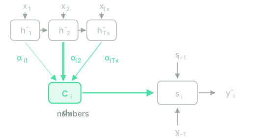
The context enters the decoder's recurrence as one more term, with its own weight matrix $\mathbf{W}_{ch} \in \mathbb{R}^{d_h \times d_h}$:

where $\mathbf{o}_{y_{i-1}}$ is the one-hot vector of $y_{i-1}$, which in training is the correct token (teacher forcing) and when generating is the one the model itself wrote at the previous step. What comes out on the right of the figure is the same as in the encoder-decoder architectureBlock 4 · Lesson 1The encoder-decoder architectureThe previous lesson's two-network architecture, put to work on a real task: translation. That brings two vocabularies instead of one, and an end-of-sequence token the model predicts for itself to decide where its output stops. It also brings the reading the rest of the block depends on: the decoder doesn't return a translation, it defines a probability over every possible one (a product of distributions, one per step), and generating means walking that product greedily. A toy Spanish-to-English translator, trained in the browser, writes sentences whose length differs from its input's, with the adjective moved in front of the noun.:

one probability for each entry of the output vocabulary. When generating, the step writes the most probable entry, and that token becomes the $y_i$ that enters from below at the next step. The context doesn't reach $\hat{\mathbf{y}}_i$ directly: it goes through $\mathbf{s}_i$ first.

The starting state, on the other hand, does change. In the encoder-decoder lessonBlock 4 · Lesson 1The encoder-decoder architectureThe previous lesson's two-network architecture, put to work on a real task: translation. That brings two vocabularies instead of one, and an end-of-sequence token the model predicts for itself to decide where its output stops. It also brings the reading the rest of the block depends on: the decoder doesn't return a translation, it defines a probability over every possible one (a product of distributions, one per step), and generating means walking that product greedily. A toy Spanish-to-English translator, trained in the browser, writes sentences whose length differs from its input's, with the adjective moved in front of the noun. the decoder started at $\mathbf{s}_0 = \mathbf{c}$, because there was one $\mathbf{c}$ and only one. Now there isn't, so we take $\mathbf{s}_0 = \mathbf{0}$, like the recurrence of the previous block. That's a choice, not a necessity (the usual alternative is to start from a learned projection of $\bar{\mathbf{h}}_{T_x}$), and nothing that follows depends on it.

With that, we can rewrite the uncomfortable line from the lesson on the encoder-decoder architectureBlock 4 · Lesson 1The encoder-decoder architectureThe previous lesson's two-network architecture, put to work on a real task: translation. That brings two vocabularies instead of one, and an end-of-sequence token the model predicts for itself to decide where its output stops. It also brings the reading the rest of the block depends on: the decoder doesn't return a translation, it defines a probability over every possible one (a product of distributions, one per step), and generating means walking that product greedily. A toy Spanish-to-English translator, trained in the browser, writes sentences whose length differs from its input's, with the adjective moved in front of the noun.:

The change looks like a subscript, but it changes what each step conditions on. The old equality claimed that everything the input had to say about any position of the output fitted in $d_h$ numbers fixed once and for all; this one claims something much weaker: that for each position, some mixture of the states will do. And since $\mathbf{c}_i$ is built from all $T_x$ states, step $i$ is conditioning on the complete source again. The assumption hasn't gone away. It has become cheap.

Where the weights come from

That leaves the question everything rests on: who decides the $\alpha_{ij}$? They can't be fixed in advance (that's exactly what was unfrozen above). Nor can they depend only on $j$, the input position (and with it the encoder state $\bar{\mathbf{h}}_j$ being weighted), because then every step would look at the same place. They have to depend on the pair: on the step $i$ the decoder has reached and on what sits at position $j$. So at step $i$ the mechanism scores $T_x$ pairs, the decoder's state against each of the encoder's states:

where $a$ is a function that returns a number (how compatible that decoder state and that encoder state are), and it uses the previous state $\mathbf{s}_{i-1}$ for a reason of order, not taste: computing $\mathbf{s}_i$ requires already having $\mathbf{c}_i$, which requires the weights, which require the scores. The latest state that exists when it's time to score is $\mathbf{s}_{i-1}$. That's why the scores come out row by row: those of step $i$ can't be computed until step $i-1$ has finished.

The scores are raw numbers that can be negative, so they have to be turned into a mixture. A softmax does that, and it's worth noticing what it runs over:

The weights come out positive because of the exponential and sum to one because of the denominator, which are the mixture's two conditions. As a bonus, the sharing is smooth: a slightly larger score takes a bit more of the weight, not all of it.

Two consequences follow, and the first is a bill. There's one score for every pair of step and position, so translating a sentence costs $T_x \cdot T_y$ evaluations of $a$: the price grows with the product of the two lengths. The fixed summary paid nothing, and that's exactly what was choking it. Still, it's worth knowing from the start that looking back doesn't come free.

The second explains why the softmax is used instead of something more direct. The natural move would be to keep the best-scored state, $\arg\max_j e_{ij}$, and save the whole sum. But that returns a position, and a position is a whole number: nudge the parameters of $a$ by a millionth and the index doesn't budge, until one day it jumps. The derivative of $\mathbf{c}_i$ with respect to those parameters is zero wherever it exists, so the loss would have no way of teaching $a$ to score better. With the softmax, $\mathbf{c}_i$ depends continuously on the scores, and the chain ruleBlock 2 · Lesson 7The chain rule, in earnestA hidden layer makes one and the same weight reach the loss by several paths at once, and the one-variable chain rule cannot cover that case. Within a path the derivatives multiply; across paths they add. Stacking those sums gives the Jacobian, and with it, differentiating a composition turns back into a matrix product. passes through the weights the same way it passes through anything else. Choosing smoothly is what makes choosing learnable.

The function $a$ is still missing, and this lesson doesn't define it. All it needs from $a$ is that it returns a number and is differentiable; what form it takes, how many parameters it carries and how those parameters are trained are the next lesson's business.

The per-step context, in NumPy

The cell takes the explorable's alignment (my numbers again) and one state per input token, and does three things. It checks the one property you can't see by looking at the map: that every row sums to one. It builds all eight contexts in one go, because mixing every row at once is a matrix product. And it repeats the calculation with the frozen alignment, so you can compare the two.

The middle column is the map read out loud, and the last two lines are the finding: with the alignment above, the eight steps receive eight different vectors, and with the frozen one they receive the same vector eight times, the state of the input's last token. The last column shows how much each step was missing, and it deserves a slow look, because not every step misses the same amount. The two small values, $0.25$ and $0.32$, belong to good and to <EOS>, the end-of-sequence token, which are the only two steps that pull from bueno, the very token the fixed summary carried inside it. The values for yesterday and book are above $1.35$. The fixed summary wasn't equally bad everywhere: it got things right where the sentence ends and wrong everywhere else, which is where it broke down in the previous lesson. Change one weight in the alpha matrix and run the cell again: the assert complains before you can look at anything, which is exactly its job.

Test your intuition

Four questions: what the softmax normalises over, what model you get by freezing the alignment, why mix instead of choosing, and how much it costs.

The mechanism is complete except for one piece, and it's the piece that decides everything else. Nobody computed this lesson's weights: I wrote them into a matrix, choosing them so that the map would show a reordering and a shared token. A real model has no one to write them for it. It has to score each pair $(\mathbf{s}_{i-1}, \bar{\mathbf{h}}_j)$ on its own, with a function that starts out knowing as little as the rest of the network and learns alongside it.

That function is $a$, and the next lesson, on Bahdanau's attention, is the one that writes it. It gives $a$ its own parameters (a small layer, with its matrix and its vector), puts it into the same gradient descent that already trains the encoder and the decoder, and derives how the gradient reaches it, which turns out to be along two routes at once. The rest of the block then shows that there's more than one reasonable way to score a pair, and that the choice between them ends up deciding what Block 5 looks like.