Implementing an MLP from scratch

Backpropagation hands over the gradient of a whole network in a single backward pass, and the previous lesson derived it without skipping a single step. What it produced, though, was a list of numbers on a screen. A printed gradient moves no weight on its own: it's an instruction (which way is down, and how much of it falls to each parameter), and somebody still has to carry that out, a thousand times over, before a network goes from answering anything at all to answering well. That loop hasn't been written in any cell of this course yet. Its four pieces have, spread across four lessons of this block, and putting them together also settles a debt open since the very beginning: the eight weights of the review neuron and the seven that separate the XOR (exclusive or) phrases were written by me, by looking at the data alone.

The place to check all this has been chosen since then. The lesson on XOR and hidden layersBlock 2 · Lesson 3XOR: why we need hidden layersFour phrases that differ only by a negation land on the corners of a square, with one class on each diagonal, and no single neuron can classify them: the pre-activation is affine, and its mean over each class works out to the same number either way. Two neurons in parallel, with a third stacked on top, can do it, because the hidden layer changes the coordinates underneath. proved that no single line leaves it's good and not bad on one side and the other two phrases on the other, then solved all four with a hidden layer whose seven numbers I picked by hand. If the loop actually works, the network has to find weights that get all four right (not necessarily mine) starting from numbers that mean nothing at all. And if it doesn't work, you'll notice immediately: with four examples and two coordinates, there's nowhere left for a fault to hide.

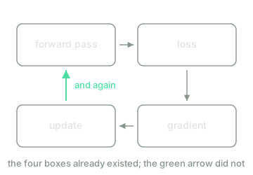
The four pieces aren't loose ends. They fall into an order, and that order closes back on itself.

From the example to the batch: the backward pass, stacked by rows

The previous lesson derived the backward pass for one example, in column vectors. The forward pass has been written for a whole batch since the lesson on the forward passBlock 2 · Lesson 4The forward pass in matrix formA whole layer collapses into one matrix product, and a whole batch fits into that same product with one row per example. That is where the transpose comes from (examples stack as rows, but an example itself is a column), and chaining those products from input to output gives you the forward pass, whose parameter cost never depends on how many examples go through at once.: one example per row in $\mathbf{X} \in \mathbb{R}^{B \times d_0}$, and from there $\mathbf{H}^{(l)} \in \mathbb{R}^{B \times d_l}$ layer by layer. The backward pass still needs that same treatment, and it comes down to two changes: one of shape, one of size.

The shape change is stacking. Call $\boldsymbol{\Delta}^{(l)} \in \mathbb{R}^{B \times d_l}$ the batch error at layer $l$: row $i$ is the $\boldsymbol{\delta}^{(l)}$ of example $i$, laid on its side, exactly the way row $i$ of $\mathbf{H}^{(l)}$ is its activation laid on its side. Capital for the batch, lower case for the example, this block's usual convention. The output layer enters exactly as before, only now with $B$ rows at once:

And the recurrence transposes whole. Take the previous lesson's version, for example $i$, $\boldsymbol{\delta}^{(l)}_i = \left(\left(\mathbf{W}^{(l+1)}\right)^{\top}\boldsymbol{\delta}^{(l+1)}_i\right) \odot \varphi^{\prime}\left(\mathbf{z}^{(l)}_i\right)$, and transpose it. Transposing a product reverses the order of its factors, and the Hadamard product works coordinate by coordinate, so it doesn't even notice:

which is row $i$ of what you're after, written using rows $i$ of $\boldsymbol{\Delta}^{(l+1)}$ and of $\mathbf{Z}^{(l)}$. Stack all $B$ of them, and you get

where what's worth noticing is what disappeared: the transpose. That's neither an oversight nor a different convention. The forward pass gained a transpose when it moved to rows ($\mathbf{W}^{(l)}\mathbf{h}$ became $\mathbf{H}\left(\mathbf{W}^{(l)}\right)^{\top}$), and the backward pass loses it for the exact same reason, since it started from a matrix that was already transposed. Both times, it's the same product read with the examples sitting in rows.

The size change is the $1/B$, and it comes straight from how the loss is defined. $\mathcal{L}$ is the mean of the $\ell$ across the $B$ examples, and differentiating a mean means taking the mean of the derivatives, so the gradient of the batch is the mean of the $B$ gradients the previous lesson would have handed you one at a time. That mean turns out to be another matrix product:

with $\mathbf{1}_B \in \mathbb{R}^{B}$ the vector of ones from the lesson on the forward passBlock 2 · Lesson 4The forward pass in matrix formA whole layer collapses into one matrix product, and a whole batch fits into that same product with one row per example. That is where the transpose comes from (examples stack as rows, but an example itself is a column), and chaining those products from input to output gives you the forward pass, whose parameter cost never depends on how many examples go through at once.. The sum over examples the previous lesson wrote out by hand is exactly the index the matrix product runs over and discards, which is why the result has the shape of $\mathbf{W}^{(l)}$ and carries no memory of $B$ at all.

With that in hand, the descent rule from the lesson on gradient descentBlock 2 · Lesson 6Gradient descentThe gradient gathers one partial derivative per parameter and points, among all possible directions, at the one that raises the loss the most; subtracting a little of it each time is the entire method. How much "a little" turns out to be decides between converging, bouncing and diverging, and the whole sum can be worked out on a parabola. doesn't change by a single letter: $\theta_{t+1} = \theta_t - \eta\,\nabla_{\theta}\mathcal{L}(\theta_t)$, applied to each matrix and each bias vector on its own. One concession, worth saying out loud: every step here looks at the entire training set (the labelled examples the network has, in this case the four phrases), exactly as that lesson did with the ten reviews. Splitting it into pieces and taking one step per piece only becomes necessary once the set grows large, and this one has all of four rows.

Everything the four-phrase network needs is on the table now: the smallest multilayer perceptron (MLP) worth trying it on, with two inputs, four hidden neurons using $\tanh$ and one output neuron with a sigmoid, that is, $L = 2$ and $d_0, d_1, d_2 = 2, 4, 1$. Its forward pass takes one line per layer,

with $\mathbf{X} \in \mathbb{R}^{4 \times 2}$ and $B = 4$, and its backward pass is the three formulas above with $L = 2$. Twelve weights and five biases: seventeen numbers that all need to go somewhere before the very first step.

Four identical neurons are a single neuron

Deciding where those seventeen numbers start is the one call no earlier formula makes, and the comfortable answer, all of them zero, fails outright. Follow the arithmetic through with that same network and seventeen zeros. Then $\mathbf{Z}^{(1)} = \mathbf{0}$, and since $\tanh(0) = 0$, also $\mathbf{H}^{(1)} = \mathbf{0}$; from there $\hat{\mathbf{Y}} = \sigma(\mathbf{0})$, which is $1/2$ for all four phrases. Feed that into the two gradients above:

the first because $\mathbf{H}^{(1)}$ is null and the second because $\mathbf{W}^{(2)}$ is. With $\boldsymbol{\Delta}^{(1)} = \mathbf{0}$, the two gradients of the first layer vanish too, so the step leaves the network exactly where it was, and the next one finds the same starting point all over again. The hidden layer will never move.

And zero isn't really the problem, it's a particular case of something much wider. Take two hidden neurons $j$ and $k$ that start out with the same input weights, the same bias and the same output weight. The forward pass gives them the same pre-activation and the same activation, $z^{(1)}_j = z^{(1)}_k$ and $h^{(1)}_j = h^{(1)}_k$; the backward pass makes them receive the same error, $\delta^{(1)}_j = \delta^{(1)}_k$; and with the same error and the same activation, all three of their gradients coincide:

Subtracting equal quantities from equal quantities preserves the equality, so the two neurons come out of the step exactly as identical as they went in. And out of the next one after that.

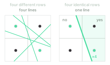
That single line is the very one from the lesson on XOR and hidden layersBlock 2 · Lesson 3XOR: why we need hidden layersFour phrases that differ only by a negation land on the corners of a square, with one class on each diagonal, and no single neuron can classify them: the pre-activation is affine, and its mean over each class works out to the same number either way. Two neurons in parallel, with a third stacked on top, can do it, because the hidden layer changes the coordinates underneath., which proved that none of them work: the hidden layer effectively has the width of one neuron, no matter how loudly $d_1$ claims four.

Seen from the seventeen numbers rather than from the plane, the equality turns into a trap shaped like a subspace. A configuration with all four neurons identical has only five real numbers dressed up as seventeen: one row of $\mathbf{W}^{(1)}$, one bias, one weight of $\mathbf{W}^{(2)}$, and $b^{(2)}$. Together they form a five-dimensional subspace sitting inside the seventeen, and the gradient always comes out tangent to it.

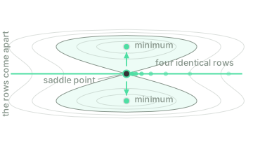
Nothing in the algorithm ever breaks that equality on its own, because everything it does is deterministic: the break has to come from outside, and the cheapest source of "different" is a random draw. Choosing those seventeen starting numbers is the initialisation, the one point in training where chance actually enters. Its role isn't quite what it looks like: it contributes no information whatsoever about the phrases, it only pulls some neurons apart from others so the gradient can push them down different paths. How large those numbers are matters too (tiny weights end up looking too much like the case above), and the third cell measures exactly that. Which scale to pick in general depends on the depth of the network, and it comes back in Block 3, on recurrent networks, once the problem stops being a minor inconvenience and becomes the whole subject.

The loop in NumPy, and the loss falling

The first cell turns the formulas above into NumPy: the forward pass, the loss and the backward pass, with no loop yet. Run it and look at the column of shapes, then the last line.

The column of shapes holds the whole division of labour: the $4$ examples show up in $\mathbf{X}$, in $\mathbf{H}^{(1)}$ and in $\hat{\mathbf{Y}}$, and in none of the three gradients, which come out with the shape of their own parameters instead. The last line checks the $1/B$ and returns zero: the four outer products from the previous lesson, averaged by hand, match the matrix product above entry for entry.

The second cell puts that into a loop and repeats it two thousand times, with $\eta = 0.5$. Run it and watch the loss fall.

The loss starts at $0.7260$ and ends at $0.0011$, and all four correct answers show up before step $25$. The debt is paid off: nobody told the network that not flips the sign of whatever follows, and the weights it found aren't even the ones I wrote in the lesson on XOR and hidden layersBlock 2 · Lesson 3XOR: why we need hidden layersFour phrases that differ only by a negation land on the corners of a square, with one class on each diagonal, and no single neuron can classify them: the pre-activation is affine, and its mean over each class works out to the same number either way. Two neurons in parallel, with a third stacked on top, can do it, because the hidden layer changes the coordinates underneath..

They're better than that: they're the same ones, rediscovered independently. Look at neurons $2$ and $4$. Their weights point in almost exactly the same direction ($(1.83,\ 1.77)$ and $(1.79,\ 1.85)$, both close to $x_1 + x_2$), their biases are opposite ($-1.80$ and $+1.80$), and so are their output weights ($-3.98$ and $+3.93$). That's the strip from the lesson on XOR and hidden layersBlock 2 · Lesson 3XOR: why we need hidden layersFour phrases that differ only by a negation land on the corners of a square, with one class on each diagonal, and no single neuron can classify them: the pre-activation is affine, and its mean over each class works out to the same number either way. Two neurons in parallel, with a third stacked on top, can do it, because the hidden layer changes the coordinates underneath.: two parallel lines and a subtraction between them. The last table confirms it: that pair contributes $+7.5$ to the two positive phrases and only $+0.2$ to the other two. And the pair $1$ and $3$ does the same on the other diagonal with the sign reversed, subtracting $6.7$ exactly where the first pair stays quiet.

What's left is deciding when to stop, and it's the flimsiest of the three decisions by far. Here I stop at a round number of steps because the curve has flattened out; I could equally well have stopped once the loss stopped falling by a thousandth, or once the norm of the gradient dropped below some threshold, and all three are rules of thumb. Correct-answer counts are no use here: by step $25$ there are already four of them, and there they stay, while the loss keeps falling by a factor of three hundred afterwards. And all three rules share a limit none of them can fix, because all three only ever look at these same four phrases.

The third cell goes back to the start of the loop and changes exactly one thing: where the weights come from. Six scales at the same seed, and below them, four genuinely identical neurons.

The first two rows of the table never budge from $0.6931$, which is $\log 2$: the network answers $0.5$ to all four phrases at the start and is still answering the same thing a thousand steps later. The second of the two is the one that actually teaches something, since its scale is $0.01$ rather than zero: the four neurons really are different from each other. What happens instead is that each layer receives a gradient multiplied by the other one's scale, and with two small factors stacked together, everything advances hundreds of times more slowly: that network isn't stuck at all, it still reaches the four phrases, only around step fifty thousand instead. At the other end, the scale $10$ starts at $4.73$ (confidently wrong) and recovers anyway: with only two layers that comes cheap, and once depth increases, it stops being cheap at all.

The last three lines show symmetry with no zeros anywhere in sight. All four neurons start with proper normal weights, only equal to one another, and a thousand steps later they're still the same row repeated four times over. The loss has fallen from $0.7240$ to $0.6931$, which is exactly what a network that answers the same thing to everything achieves: four neurons working as one, and one neuron cannot do the job.

Test your intuition

Two questions (why zero freezes the network, and what can actually be read off a loss curve), plus a challenge that is the whole loop.

The network gets the four phrases it has seen right, and there is no fifth to check it against. That isn't a defect of the training, it's that here getting it right and genuinely learning are indistinguishable, since with only four examples, memorising the answer and understanding the rule produce exactly the same numbers. Nothing this loop prints says what the network would do with not that good, and the loop has no way of ever finding out.

There's also a debt this whole business with the weights has left sitting in plain sight. I invented the two input coordinates myself: whether not appears, and whether the evaluative word is good or bad, are two questions somebody had to formulate after reading the four phrases, and an arbitrary piece of text doesn't arrive already packaged into two numbers. It did arrive, though, as the bag of words from the previous block. Mounting this same loop on a few hundred reviews represented that way, measuring accuracy for the first time on reviews the network has never seen, and finding out what's left of it, is the next lesson, the sentiment classification project.