GRU: the simplified version

26 min read

So far this block has moved forward by asking what each network was missing: the vanilla recurrent neural network (RNN) lacked a memory that could survive distance, and the previous lesson's long short-term memory (LSTM), on gated memory, supplied one. But it came at a cost: four times the weights of a vanilla RNN, and a second vector hauled through every step. And the lesson itself ended by doubting that every one of its gates was needed. Once an architecture works, the question is no longer what it's missing, but what it could do without.

Real simplification doesn't mean removing pieces until something breaks; it means removing them without losing what they paid for. And what the LSTM paid for (the one thing that justified all that machinery) was the return path, the route along which the gradient comes back intact across many steps. Every cut has to be checked against it: if merging gates or dropping states loses that path, the simplification has thrown away exactly what mattered. The gated recurrent unit (GRU) is the cut that passes the test, which is why it became the standard alternative to the LSTM in practice: a quarter fewer weights, one state, and (almost always, though not always) the same result.

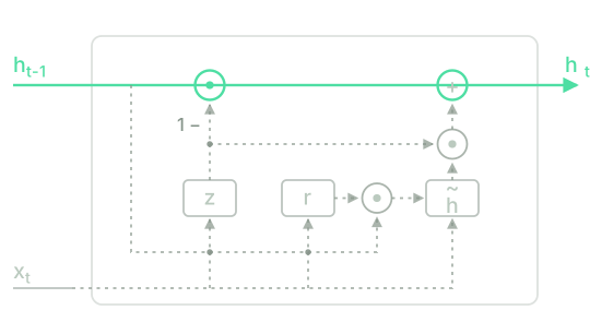
The cut comes down to two ideas. The first fuses the forget gate and the input gate: instead of deciding separately how much to keep and how much to write, the GRU uses a single control (the update gate) that says how much to replace, and whatever it doesn't replace, it keeps. The state stops being a sum that can grow without limit and becomes a mix, a point partway between what was there and what's being proposed; and a mix of bounded things stays bounded, so the output gate that trimmed the LSTM's state before showing it is no longer needed.

The second idea is a small new gate, the reset gate, which leaves the memory alone and acts on the candidate instead: it lets the candidate ignore the previous state when what needs writing now carries nothing over from before (at the start of a new sentence, say). With those two gates, and a single state that serves as both memory and output, the second vector disappears: there's no longer a cell state hidden behind the one on display.

Before the formulas, take one more look at the LSTM the GRU simplifies. Step through it and watch the first two rows (the forget gate and the input gate) move independently: those are the two the GRU is about to tie into one.

The previous lesson's LSTM step, seen with fresh eyes. Watch the first two rows, the forget gate and the input gate: they move independently, and that's exactly the freedom the GRU ties into a single gate. The last row, how much of c₁ survives, is the guarantee the simplification must not lose.

Keeping and writing with a single gate

Start with the line that changes everything. The LSTM's cell added two terms with independent gates, $\mathbf{c}_t = \mathbf{f}_t \odot \mathbf{c}_{t-1} + \mathbf{i}_t \odot \tilde{\mathbf{c}}_t$ ; the GRU works directly on the hidden state $\mathbf{h}_t \in \mathbb{R}^{d_h}$ (there's no second vector) and ties the two gates into one:

\mathbf{h}_t = (1 - \mathbf{z}_t) \odot \mathbf{h}_{t-1} + \mathbf{z}_t \odot \tilde{\mathbf{h}}_t,

where $\mathbf{z}_t \in (0,1)^{d_h}$ is the update gate and $\tilde{\mathbf{h}}_t \in (-1,1)^{d_h}$ is the candidate, the state the step proposes. Coordinate by coordinate, it's a weighted average of old and new: $z_{t,j} = 0$ leaves $h_{t,j}$ equal to $h_{t-1,j}$ (it keeps), and $z_{t,j} = 1$ replaces it entirely with the candidate (it writes). There's no way to do both at once, and that's precisely the freedom the LSTM had and the GRU gives up: there, $\mathbf{f}_t$ and $\mathbf{i}_t$ could both open and accumulate. In exchange, an average of bounded numbers can't overflow, which is why the GRU shows its state as it is, without the output gate or the $\tanh$ that trimmed the LSTM's state before letting it out.

The update gate is computed like every gate in the previous lesson, as a sigmoid layer over the token and the previous state:

\mathbf{z}_t = \sigma\left(\mathbf{W}_{xz}\mathbf{x}_t + \mathbf{W}_{hz}\mathbf{h}_{t-1} + \mathbf{b}_z\right),

with $\mathbf{W}_{xz} \in \mathbb{R}^{d_h \times d_{\text{model}}}$ , $\mathbf{W}_{hz} \in \mathbb{R}^{d_h \times d_h}$ and $\mathbf{b}_z \in \mathbb{R}^{d_h}$ : the same shapes as the recurrence in the lesson on the vanilla RNNBlock 3 · Lesson 2The vanilla RNNOne matrix applied at every position, and a state carried from each step to the next. That's enough to keep the length of the text out of every weight's shape: the same network reads two tokens or forty without padding or truncating anything, what it learns at position 2 works unchanged at position 8, and two sentences with the same tokens in a different order are no longer the same input..

That leaves the candidate, and this is where the second gate comes in. In the LSTM, the candidate always read the whole previous state; the GRU puts a filter in front of it, the reset gate $\mathbf{r}_t$ , which decides how much of that state the candidate gets to see:

\mathbf{r}_t = \sigma\left(\mathbf{W}_{xr}\mathbf{x}_t + \mathbf{W}_{hr}\mathbf{h}_{t-1} + \mathbf{b}_r\right), \qquad \tilde{\mathbf{h}}_t = \tanh\left(\mathbf{W}_{xh}\mathbf{x}_t + \mathbf{W}_{hh}\left(\mathbf{r}_t \odot \mathbf{h}_{t-1}\right) + \mathbf{b}_h\right).

That $\mathbf{r}_t \odot \mathbf{h}_{t-1}$ is the only thing that sets this candidate apart from a vanilla RNN step: with $\mathbf{r}_t = \mathbf{1}$ the candidate is exactly the recurrence from the lesson on the vanilla RNNBlock 3 · Lesson 2The vanilla RNNOne matrix applied at every position, and a state carried from each step to the next. That's enough to keep the length of the text out of every weight's shape: the same network reads two tokens or forty without padding or truncating anything, what it learns at position 2 works unchanged at position 8, and two sentences with the same tokens in a different order are no longer the same input., and with $\mathbf{r}_t = \mathbf{0}$ it's computed from the token alone, as if the sequence started there. Keep the two gates apart: $\mathbf{z}_t$ decides whether the state gets updated, while $\mathbf{r}_t$ decides what the candidate looks at when making its proposal. One governs the memory, the other the candidate.

Here are the three pieces together, with $\mathbf{h}_0 = \mathbf{0}$ for the same reason as in the RNN and the LSTM:

\begin{aligned} \mathbf{z}_t &= \sigma\left(\mathbf{W}_{xz}\mathbf{x}_t + \mathbf{W}_{hz}\mathbf{h}_{t-1} + \mathbf{b}_z\right), & \mathbf{r}_t &= \sigma\left(\mathbf{W}_{xr}\mathbf{x}_t + \mathbf{W}_{hr}\mathbf{h}_{t-1} + \mathbf{b}_r\right), \\ \tilde{\mathbf{h}}_t &= \tanh\left(\mathbf{W}_{xh}\mathbf{x}_t + \mathbf{W}_{hh}\left(\mathbf{r}_t \odot \mathbf{h}_{t-1}\right) + \mathbf{b}_h\right), & \mathbf{h}_t &= (1 - \mathbf{z}_t) \odot \mathbf{h}_{t-1} + \mathbf{z}_t \odot \tilde{\mathbf{h}}_t. \end{aligned}

One step of a GRU. A green line, the hidden state, runs across the top from side to side: it enters as h sub t minus one, leaves as h sub t, and meets only two circles along the way, one for a product and one for a sum. Below it sit three small boxes labelled z, r, and h with a tilde. Box z feeds up through a "1 −" into the product circle on the green line, and a branch from it runs right to another product circle below the line, where it meets h with a tilde; only the output of that circle rises to the sum. Before the first circle, a dotted line carrying the previous state drops from the green line and feeds z and r, together with the vector of the token. Box h with a tilde does not read that line directly, but through a third product circle where r filters it. On the right there is no output gate and no tanh: the green line is both the memory and the output. — The four equations above, drawn out: the LSTM's green path, now travelled by the hidden state itself, which leaves on the right exactly as it is, with no output gate and no tanh. A single gate, z, controls it, keeping on one side through 1 − z and writing on the other; r never touches it, and only filters what the candidate reads from the past.

Three pieces (two gates and a candidate), each with exactly the shape of the recurrence in the lesson on the vanilla RNNBlock 3 · Lesson 2The vanilla RNNOne matrix applied at every position, and a state carried from each step to the next. That's enough to keep the length of the text out of every weight's shape: the same network reads two tokens or forty without padding or truncating anything, what it learns at position 2 works unchanged at position 8, and two sentences with the same tokens in a different order are no longer the same input.: six matrices and three biases, $3\left(d_h \cdot d_h + d_h \cdot d_{\text{model}} + d_h\right)$ weights. That's three quarters of the LSTM's four groups; and as with the LSTM, $T$ appears in none of the shapes, so the GRU reads any length with a single set of weights.

Why the return path survives the cut

The whole lesson hangs on one check: that the return path (the one the LSTM paid for, and whose necessity the lesson on the vanishing gradientBlock 3 · Lesson 4The vanishing gradientMultiplying by the same recurrent matrix at every step makes the gradient exponential in the distance it travels. What guarantees that it vanishes is γ·σ_max < 1, the steepest tanh slope times the largest singular value of W_hh; the spectral radius only sets the pace of the matrix on its own. Gradient clipping stops the explosion but can't rescue a gradient that has already vanished, and that's what will force a change of architecture. explained) is still standing with one state instead of two. Look at the last equation coordinate by coordinate, which is where the meaning of the $\odot$ becomes visible:

h_{t,j} = (1 - z_{t,j})\,h_{t-1,j} + z_{t,j}\,\tilde{h}_{t,j}.

Along this path, coordinate $j$ of the new state depends on coordinate $j$ of the old one and on no other: there's no matrix to mix them. Differentiating along the direct path while holding the gates and the candidate still (I'll come back to this),

\frac{\partial h_{t,j}}{\partial h_{t-1,j}} = 1 - z_{t,j},

a number, not a matrix. Chain it backwards to a distant step $k$ , the way the lesson on the vanishing gradientBlock 3 · Lesson 4The vanishing gradientMultiplying by the same recurrent matrix at every step makes the gradient exponential in the distance it travels. What guarantees that it vanishes is γ·σ_max < 1, the steepest tanh slope times the largest singular value of W_hh; the spectral radius only sets the pace of the matrix on its own. Gradient clipping stops the explosion but can't rescue a gradient that has already vanished, and that's what will force a change of architecture. chained the recurrence, and what arrives along the direct path is a product of those numbers:

\frac{\partial \ell}{\partial h_{k,j}} = \left(\prod_{t=k+1}^{T}\left(1 - z_{t,j}\right)\right)\frac{\partial \ell}{\partial h_{T,j}} + \left(\text{what comes in through the gates}\right).

It's the LSTM's $\prod f_{t,j}$ letter for letter, with $1 - z_{t,j}$ in place of $f_{t,j}$ : the closed update gate ( $z_{t,j} \to 0$ ) plays the role of the open forget gate. And the same thing holds as before ( $1 - z_{t,j} = 1$ is reachable and stable, because a saturated sigmoid stays flat at its extreme), so a coordinate the network learns not to update multiplies by $1$ for as many steps as needed. Compared with the $\left(\gamma\,\sigma_{\max}\right)^{T-k}$ of the lesson on the vanishing gradientBlock 3 · Lesson 4The vanishing gradientMultiplying by the same recurrent matrix at every step makes the gradient exponential in the distance it travels. What guarantees that it vanishes is γ·σ_max < 1, the steepest tanh slope times the largest singular value of W_hh; the spectral radius only sets the pace of the matrix on its own. Gradient clipping stops the explosion but can't rescue a gradient that has already vanished, and that's what will force a change of architecture., the base is no longer a property of one matrix shared by everything; it's a number per coordinate and per step that the network computes.

See what "holding the gates still" left out

$\mathbf{z}_t$ , $\mathbf{r}_t$ and $\tilde{\mathbf{h}}_t$ are computed from $\mathbf{h}_{t-1}$ , so the full derivative adds, to the direct path's $1 - z_{t,j}$ , the paths that run through the two gates and through the candidate. Every one of them crosses a $\mathbf{W}_{h\ast}$ and an activation mask, and they vanish the same way as the paths in the lesson on the vanishing gradientBlock 3 · Lesson 4The vanishing gradientMultiplying by the same recurrent matrix at every step makes the gradient exponential in the distance it travels. What guarantees that it vanishes is γ·σ_max < 1, the steepest tanh slope times the largest singular value of W_hh; the spectral radius only sets the pace of the matrix on its own. Gradient clipping stops the explosion but can't rescue a gradient that has already vanished, and that's what will force a change of architecture..

Their vanishing breaks nothing, and the reasoning is the same as for the LSTM. Those paths adjust how the decision is made at each step, and a decision at this step relies on what's nearby; the gradient that has to arrive from far away travels the direct path, and that path crosses no matrix. The GRU doesn't eliminate the product from the lesson on the vanishing gradientBlock 3 · Lesson 4The vanishing gradientMultiplying by the same recurrent matrix at every step makes the gradient exponential in the distance it travels. What guarantees that it vanishes is γ·σ_max < 1, the steepest tanh slope times the largest singular value of W_hh; the spectral radius only sets the pace of the matrix on its own. Gradient clipping stops the explosion but can't rescue a gradient that has already vanished, and that's what will force a change of architecture.: it moves it off the long path and leaves it on the short ones.

Two concessions close the account, the same two as for the LSTM. If the network learns $z_{t,j}$ around $0.3$ , the product sinks as it did in the RNN, except that now it's because the network chose to, not because the architecture forces it. And explosion is still possible along the paths in the box above, so the GRU is trained with gradient clipping like everything before it. The additive path doesn't hand out a guarantee; it puts within reach an option that was out of reach before.

The GRU, step by step, in NumPy

One cell. It transcribes the four-equation block and runs it on a short sequence with two different update-gate biases, to see how much of $\mathbf{h}_1$ reaches $\mathbf{h}_6$ along the direct path.

Once again the weights come from a generator with a fixed seed and are untrained, so the gates don't mean anything yet. What I did set by hand is the bias $\mathbf{b}_z$ : remember that keeping means $z \to 0$ , so a negative bias is what nudges the network towards remembering (the mirror image of the LSTM's positive $\mathbf{b}_f$ ). Look at the last line of each block.

import numpy as np

d_model, d_h, T = 4, 3, 6
X = np.random.default_rng(1).normal(size=(T, d_model)) * 0.5


def sigmoid(z):
  return 1.0 / (1.0 + np.exp(-z))


def weights(update_bias):
  rng = np.random.default_rng(0)                 # the same weights in both cases
  return {k: (rng.normal(size=(d_h, d_model)) * 0.5,
              rng.normal(size=(d_h, d_h)) * 0.5,
              np.full(d_h, b))
          for k, b in [("z", update_bias), ("r", 0.0), ("h", 0.0)]}


def step(P, h, x):
  def pre(k, state):
      Wx, Wh, b = P[k]
      return Wx @ x + Wh @ state + b
  z = sigmoid(pre("z", h))
  r = sigmoid(pre("r", h))
  cand = np.tanh(pre("h", r * h))                # the candidate reads r (*) h_{t-1}
  h = (1 - z) * h + z * cand                     # the additive path, tied
  return h, z, r


for bias in [0.0, -3.0]:
  P = weights(bias)
  h, kept = np.zeros(d_h), []
  print("b_z = %.0f" % bias)
  print("  t      z_t              r_t              h_t")
  for t, x in enumerate(X, 1):
      h, z, r = step(P, h, x)
      kept.append(1 - z)
      print("  %d  %s %s %s" % (t, np.round(z, 2), np.round(r, 2), np.round(h, 2)))
  print("  what survives of h_1 in h_6:", np.round(np.prod(kept[1:], axis=0), 3))

numpy

The first run downloads the Python interpreter (~15 MB). After that it stays in the browser cache and is reused across every lesson.

Both gates live in $(0,1)$ , and each coordinate gets its own value (where two print the same, they differ beyond the second decimal place). Compare the two blocks by their last lines. With $\mathbf{b}_z = 0$ , the update gate hovers around $0.5$ , half the state is replaced at every step, and about $3\%$ of $\mathbf{h}_1$ reaches $\mathbf{h}_6$ ; with $\mathbf{b}_z = -3$ , it hovers around $0.05$ , almost nothing gets updated, and $77\%$ survives, with the same weights and the same sequence. Hence the habit of initialising $\mathbf{b}_z$ to a negative value, for the same reason as a positive $\mathbf{b}_f$ in the LSTM: it's cheaper for the network to learn to write than to learn to remember. And notice the price of the shortcut: with $\mathbf{b}_z = -3$ the state barely moves ( $\mathbf{h}_t$ stays in the hundredths), because keeping and writing are the same control, and asking it to keep means asking it to barely write.

Test your intuition

Four questions: what the update gate ties together and what it gives up, what the reset gate does without touching the memory, what the architecture costs, and what the GRU takes from the LSTM and what it leaves behind.

What does the GRU gain, and what does it lose, by replacing the LSTM's forget and input gates with a single update gate $\mathbf{z}_t$ ?

It gains a new state that's a mix of the old one and the candidate (

(1-\mathbf{z}_t)

keeps,

\mathbf{z}_t

writes, and the two add up to one), so it stays bounded without an output gate to trim it. It loses the ability to keep and write at the same time: tying them together as

\mathbf{z}_t

and

1-\mathbf{z}_t

means that writing more always means keeping less.It gains one weight fewer per coordinate and loses nothing, because in the LSTM the forget gate and the input gate were always one minus the other.It gains speed, because

\mathbf{z}_t

is computed with

\tanh

instead of

\sigma

, and loses nothing.It gains memory, because with one gate fewer there are fewer paths along which the gradient can vanish; it loses the ability to forget.

The reset gate $\mathbf{r}_t$ multiplies the previous state inside the candidate: $\tilde{\mathbf{h}}_t = \tanh\left(\mathbf{W}_{xh}\mathbf{x}_t + \mathbf{W}_{hh}\left(\mathbf{r}_t \odot \mathbf{h}_{t-1}\right) + \mathbf{b}_h\right)$ . With $\mathbf{r}_t \approx \mathbf{0}$ , what happens?

The candidate stops looking at the previous state and is computed from the token alone, as if the sequence started there. The stored state isn't erased: that's up to

\mathbf{z}_t

, not

\mathbf{r}_t

.The state is set to zero, because reset means restarting the memory.The state stops updating:

\mathbf{r}_t \approx \mathbf{0}

leaves

\mathbf{h}_t = \mathbf{h}_{t-1}

.Nothing visible, because

\mathbf{r}_t

and

\mathbf{z}_t

do the same job and cancel out.

Take a GRU with a state of $d_h = 64$ coordinates reading embeddings of $d_{\text{model}} = 128$ , the same dimensions as the previous lesson's LSTM. How many weights do its six matrices and three biases add up to?

A margin of ±0 is accepted.

Tick everything that is true of the GRU compared with the LSTM.

Select every correct option. This is graded all-or-nothing: there is no partial credit.

It keeps the return path the LSTM gained: along the direct path the gradient is multiplied by

(1-z_{t,j})

, one number per coordinate and per step that the network can hold close to

1

, instead of by the power of a shared matrix.It still needs gradient clipping, because the candidate and both gates cross their

\mathbf{W}_{h\ast}

matrices the way the vanilla RNN does, so explosion is still possible.It's always better than the LSTM, because with fewer weights it generalises better.It needs to fix

T_{\max}

and pad, because with a single state it can no longer read sequences of any length.

And then the full step, written by you: the recurrence from the vanilla RNNBlock 3 · Lesson 2The vanilla RNNOne matrix applied at every position, and a state carried from each step to the next. That's enough to keep the length of the text out of every weight's shape: the same network reads two tokens or forty without padding or truncating anything, what it learns at position 2 works unchanged at position 8, and two sentences with the same tokens in a different order are no longer the same input. wrapped in two gates.

Write one GRU step: gru_step(h, x, P) takes the previous state, the current token's vector, and a dictionary P holding the weights of the three pieces (P["z"], P["r"] and P["h"], each a triple (Wx, Wh, b)). It returns h_new.

The two gates are sigmoids over the token and the previous state; the candidate is a $\tanh$ that reads $\mathbf{r}_t \odot \mathbf{h}_{t-1}$ instead of the bare $\mathbf{h}_{t-1}$ , and the new state is the mix $(1-\mathbf{z}_t)\odot\mathbf{h}_{t-1} + \mathbf{z}_t\odot\tilde{\mathbf{h}}_t$ . Compute both gates from the incoming state, not the one you're about to return. Don't write into the arrays you receive.

The first run downloads the Python interpreter (~15 MB); after that it stays in the browser cache. This challenge is much easier to solve on a physical keyboard: on a phone, read it and come back later.

With the GRU and the LSTM, the block now has two ways of giving a network memory, and both rest on the same discovery: a path along which the state moves forward by adding, without crossing a matrix, is the only thing that lets the gradient come back from far away. But knowing how to build a cell isn't the same as having built something with it. In this entire block, no network has yet read a text from start to finish and produced language of its own: we've derived the machinery and never switched it on.

Switching it on is the job of the next lesson, a project that builds a character-level language model. It combines the vanilla RNN and backpropagation through time (BPTT) in a network that trains on a few thousand characters and then generates new text, character by character. The result will be bad (and I won't sugar-coat it when it is), it will run in your browser in a few seconds, and it will be the first time in the course that something writes.

Was this helpful?