Seq2seq: from sequence to sequence

25 min read

The previous lesson's character-level model can carry on a text: give it an opening and it keeps going, character by character, for as long as you let it. But carrying on is all it does. Plenty of tasks have a different shape: shortening a paragraph into a headline, correcting a line full of typos, turning a date written out in words into digits. In each of them one sequence goes in and another comes out, and the second isn't a continuation of the first, nor does it need to be the same length. That shape is what this lesson builds.

It's called a sequence-to-sequence model (seq2seq for short), and the idea fits in a sentence: two networks instead of one. The first, the encoder, reads the input sequence from start to finish and compresses it into a vector; the second, the decoder, starts from that vector and writes the output sequence one token at a time, the way the previous lesson's model wrote. Nothing passes between them except that vector: everything the encoder took from the input has to fit in there.

Take the simplest task with this shape: reversal. The input is live and the output is evil, the same string read backwards. To write the first letter of the output (the e), the decoder needs to know which letter the input ended on; to write the last (the l), it needs to remember the first. So to reverse a string, you have to have read all of it before you start writing, and that's exactly what the split into two networks reflects. The encoder reads live to the end and leaves its summary; only then does the decoder start producing evil.

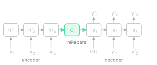
Everything the encoder read from the input crosses to the decoder at a single point, the context vector c. Whether the input is three tokens or thirty, the decoder receives the same handful of numbers.

That summary is the encoder's last state, and it has a name: the context vector, $\mathbf{c}$ . It's a vector of fixed size (exactly as many coordinates as the state, not one more), and it's the only part of the input the decoder ever gets to see. The decoder never looks at live again: it starts from $\mathbf{c}$ and writes from there, feeding itself what it produces, the way the previous lesson's model generated text.

The encoder summarises, the decoder writes

Both networks are the vanilla recurrent neural network (RNN)Block 3 · Lesson 2The vanilla RNNOne matrix applied at every position, and a state carried from each step to the next. That's enough to keep the length of the text out of every weight's shape: the same network reads two tokens or forty without padding or truncating anything, what it learns at position 2 works unchanged at position 8, and two sentences with the same tokens in a different order are no longer the same input., with nothing new in the recurrence; the only novelty is how they're chained together. The encoder reads the input tokens $\mathbf{x}_1, \dots, \mathbf{x}_{T_x}$ (each $\mathbf{x}_j$ being the one-hot vector of the $j$ -th symbol, as in the previous lesson) and updates its state:

\bar{\mathbf{h}}_j = \tanh\left(\mathbf{W}^{\text{enc}}_{xh}\mathbf{x}_j + \mathbf{W}^{\text{enc}}_{hh}\bar{\mathbf{h}}_{j-1} + \mathbf{b}^{\text{enc}}_h\right),

with $\bar{\mathbf{h}}_0 = \mathbf{0}$ . The bar over $\bar{\mathbf{h}}_j$ marks it as the encoder's state, so it can't be confused with the decoder's; the superscript $\text{enc}$ does the same for its weights, and it isn't a layer index (the encoder has no layers to number) but a label saying which network the weights belong to. When the encoder finishes reading, its last state is the context vector:

\mathbf{c} = \bar{\mathbf{h}}_{T_x} \in \mathbb{R}^{d_h}.

Notice the size of $\mathbf{c}$ : $d_h$ coordinates, the same as the state, and that number doesn't depend on $T_x$ . A three-token input and a thirty-token input produce a $\mathbf{c}$ of the same size.

The decoder is another RNN, with its own weights, that picks up where the encoder left off: its initial state is $\mathbf{s}_0 = \mathbf{c}$ . From there it produces the output step by step. At step $i$ it reads a token (at the first step <GO>, the symbol the decoder starts from, and after that the previous token) and updates its state:

\mathbf{s}_i = \tanh\left(\mathbf{W}^{\text{dec}}_{xh}\mathbf{o}_{u_{i-1}} + \mathbf{W}^{\text{dec}}_{hh}\mathbf{s}_{i-1} + \mathbf{b}^{\text{dec}}_h\right),

where $\mathbf{o}_{u_{i-1}}$ is the one-hot vector of the token $u_{i-1}$ fed in at position $i$ . Each state produces a distribution over the next symbol, as in the previous lesson's language model:

\hat{\mathbf{y}}_i = \text{softmax}\left(\mathbf{W}_{hy}\mathbf{s}_i + \mathbf{b}_y\right),

and the loss adds one cross-entropy per output position, averaged per token:

\ell = \frac{1}{T_y}\sum_{i=1}^{T_y} -\log \hat{y}_{i,\,y_i},

where $y_i$ is the symbol that really belongs at position $i$ , and $T_y$ is the length of the output, which needn't equal $T_x$ . What matters is where that loss lives: only in the decoder. The encoder predicts nothing at any of its positions, so it contributes not a single term to $\ell$ . In the previous lesson's model every position had its own output and its own loss term; here, half the network has neither.

One detail about the token $u_{i-1}$ the decoder reads at each step. During training it's given the correct symbol (the one from the real output, even if the decoder got its own prediction wrong); this is called teacher forcing, and it makes training more stable. During generation there's no correct answer to give it, so its own output is fed back in. It's the same split between training and generating as in the previous lesson, with <GO> at the start instead of a space.

How the encoder learns with no output of its own

If the encoder has no loss, where does its gradient come from? From a single place, and that's what lets this model train end to end despite being two networks. The backward pass starts at the only loss there is, the decoder's, and step for step it's the one from the lesson on the character-level language modelBlock 3 · Lesson 7Project: a character-level language modelThe vanilla RNN and BPTT, combined in a network that predicts the next character at every position: a text of T characters is T examples stacked together, and the label at each step comes for free, since it's the character that comes next. It trains with gradient clipping on a few thousand characters (for only a few steps, to fit in the browser) and then writes, feeding back what it samples. The loss falls from ln 26 to around 2.5 and the text goes from noise to broken English (real short words, long near-words, not one sentence that means anything): that's what a character model learns, and saying so outright is the lesson., without a line changed: each position starts an error from its output and transports it to the previous step. What's new happens at the end of that pass. The decoder's first state is $\mathbf{s}_0 = \mathbf{c}$ , so once the error has finished crossing the decoder backwards, it leaves a gradient on the context vector:

\nabla_{\mathbf{c}}\ell = \left(\mathbf{W}^{\text{dec}}_{hh}\right)^{\top}\boldsymbol{\delta}_1,

where $\boldsymbol{\delta}_1$ is the error at the decoder's first step, the same quantity as in the lesson on the character-level language modelBlock 3 · Lesson 7Project: a character-level language modelThe vanilla RNN and BPTT, combined in a network that predicts the next character at every position: a text of T characters is T examples stacked together, and the label at each step comes for free, since it's the character that comes next. It trains with gradient clipping on a few thousand characters (for only a few steps, to fit in the browser) and then writes, feeding back what it samples. The loss falls from ln 26 to around 2.5 and the text goes from noise to broken English (real short words, long near-words, not one sentence that means anything): that's what a character model learns, and saying so outright is the lesson.. That $\nabla_{\mathbf{c}}\ell$ is the only gradient the encoder receives, and it's all the encoder needs: since $\mathbf{c} = \bar{\mathbf{h}}_{T_x}$ , it's exactly the gradient on the encoder's last state, and from there the encoder runs its own backpropagation through time (BPTT), as if $\nabla_{\mathbf{c}}\ell$ had come from an output at its last step. Spread backwards over its $T_x$ steps, that single gradient adjusts $\mathbf{W}^{\text{enc}}_{hh}$ , $\mathbf{W}^{\text{enc}}_{xh}$ and $\mathbf{b}^{\text{enc}}_h$ .

The limit is already visible here. The whole decoder hangs off $\mathbf{c}$ , and the whole encoder is corrected through $\mathbf{c}$ : if some part of the input didn't make it into those $d_h$ coordinates, the decoder can't use it, and the gradient can't ask for it to be kept. The longer the input, the more has to be squeezed into the same vector.

See the full backward pass, from the decoder to the encoder

The decoder's backward pass is the one from the lesson on the character-level language modelBlock 3 · Lesson 7Project: a character-level language modelThe vanilla RNN and BPTT, combined in a network that predicts the next character at every position: a text of T characters is T examples stacked together, and the label at each step comes for free, since it's the character that comes next. It trains with gradient clipping on a few thousand characters (for only a few steps, to fit in the browser) and then writes, feeding back what it samples. The loss falls from ln 26 to around 2.5 and the text goes from noise to broken English (real short words, long near-words, not one sentence that means anything): that's what a character model learns, and saying so outright is the lesson., with $\mathbf{s}$ in place of $\mathbf{h}$ : the error at the pre-activation of each position is

\boldsymbol{\delta}_i = \left(\mathbf{1} - \mathbf{s}_i \odot \mathbf{s}_i\right) \odot \left(\mathbf{W}_{hy}^{\top}\left(\hat{\mathbf{y}}_i - \mathbf{y}_i\right) + \left(\mathbf{W}^{\text{dec}}_{hh}\right)^{\top}\boldsymbol{\delta}_{i+1}\right),

with $\boldsymbol{\delta}_{T_y+1} = \mathbf{0}$ . After crossing all $T_y$ steps, the transport reaches $\mathbf{s}_0 = \mathbf{c}$ and stops there: $\nabla_{\mathbf{c}}\ell = (\mathbf{W}^{\text{dec}}_{hh})^{\top}\boldsymbol{\delta}_1$ . That vector kicks off the encoder's backward pass, which is the one from the lesson on BPTTBlock 3 · Lesson 3Backpropagation through timeRecurrence shares one matrix across every position, and that changes what its gradient looks like. Backpropagation through time is the previous block's backward pass with the layers laid out along time: one error per step, carried from the end back to the start by the same W_hh, and a gradient that, because that matrix is reused at every position, is the sum of what each step asks of it. This lesson derives it in full and checks it, number by number, against a numerical probe. but with no output term (the encoder makes no prediction at any step, so the term with $\hat{\mathbf{y}}$ disappears and only the transport is left):

\bar{\boldsymbol{\delta}}_j = \left(\mathbf{1} - \bar{\mathbf{h}}_j \odot \bar{\mathbf{h}}_j\right) \odot \left(\mathbf{W}^{\text{enc}}_{hh}\right)^{\top}\bar{\boldsymbol{\delta}}_{j+1},

starting at the last step with $\bar{\boldsymbol{\delta}}_{T_x} = \left(\mathbf{1} - \mathbf{c} \odot \mathbf{c}\right) \odot \nabla_{\mathbf{c}}\ell$ . That single entry point, $\mathbf{c}$ , is the encoder's only contact with the loss.

Reversing sequences in NumPy

Now to train a seq2seq on the toy task: reversing strings of symbols. It's a toy on purpose (real translation doesn't fit in the browser), but it has the whole shape of the problem: two networks, a context vector between them, and an output that isn't a continuation of the input. The alphabet is six letters, plus a <GO> symbol that only ever enters the decoder, to get it started. Each example is a random string of 3 to 7 letters, paired with its reverse. The cell builds the two networks, chains the two backward passes (the decoder's and, hanging off $\mathbf{c}$ , the encoder's) and trains. Watch the loss per character it prints every few hundred steps.

import numpy as np

# Toy task: read a string of letters and write it backwards.
V = list("abcdef")                 # the 6 letters: the encoder's input and the decoder's output
GO = 6                             # start symbol; it only enters the decoder, never predicted
n_v, n_sym = 7, 6                  # 7 inputs (letters + GO); 6 output classes
d_h, eta, kappa, iters = 64, 0.10, 5.0, 1200

rng = np.random.default_rng(0)     # fixed seed: you'll see these numbers
sc = 0.1
Wxh_e = rng.normal(size=(d_h, n_v)) * sc; Whh_e = rng.normal(size=(d_h, d_h)) * sc; bh_e = np.zeros(d_h)
Wxh_d = rng.normal(size=(d_h, n_v)) * sc; Whh_d = rng.normal(size=(d_h, d_h)) * sc; bh_d = np.zeros(d_h)
Why = rng.normal(size=(n_sym, d_h)) * sc; by = np.zeros(n_sym)
weights = [Wxh_e, Whh_e, bh_e, Wxh_d, Whh_d, bh_d, Why, by]


def train_step(x, y):                                  # x: the source; y: the source reversed
  L = len(x)
  He = np.zeros((d_h, L)); h = np.zeros(d_h)         # --- encoder: reads and summarises ---
  for j in range(L):
      h = np.tanh(Wxh_e[:, x[j]] + Whh_e @ h + bh_e); He[:, j] = h
  c = h                                              # context vector: the last state
  dec_in = np.concatenate(([GO], y[:-1]))            # decoder with teacher forcing: GO, y1, ..., y_{L-1}
  S = np.zeros((d_h, L)); P = np.zeros((n_sym, L)); s = c.copy(); loss = 0.0
  for i in range(L):                                 # --- decoder: writes from c ---
      s = np.tanh(Wxh_d[:, dec_in[i]] + Whh_d @ s + bh_d); S[:, i] = s
      o = Why @ s + by; o -= o.max(); p = np.exp(o); p /= p.sum(); P[:, i] = p
      loss -= np.log(p[y[i]] + 1e-12)
  gWhy = np.zeros_like(Why); gby = np.zeros_like(by)  # --- decoder backward pass ---
  gWxh_d = np.zeros_like(Wxh_d); gWhh_d = np.zeros_like(Whh_d); gbh_d = np.zeros_like(bh_d)
  ds = np.zeros(d_h)
  for i in reversed(range(L)):
      dO = P[:, i].copy(); dO[y[i]] -= 1.0
      gWhy += np.outer(dO, S[:, i]); gby += dO
      dp = (1 - S[:, i] ** 2) * (Why.T @ dO + ds)
      s_prev = S[:, i - 1] if i > 0 else c
      gWhh_d += np.outer(dp, s_prev); gWxh_d[:, dec_in[i]] += dp; gbh_d += dp
      ds = Whh_d.T @ dp
  gWxh_e = np.zeros_like(Wxh_e); gWhh_e = np.zeros_like(Whh_e); gbh_e = np.zeros_like(bh_e)
  dh = ds                                            # the only link: the gradient at c
  for j in reversed(range(L)):                       # --- encoder backward pass ---
      dp = (1 - He[:, j] ** 2) * dh
      h_prev = He[:, j - 1] if j > 0 else np.zeros(d_h)
      gWhh_e += np.outer(dp, h_prev); gWxh_e[:, x[j]] += dp; gbh_e += dp
      dh = Whh_e.T @ dp
  return loss / L, [g / L for g in (gWxh_e, gWhh_e, gbh_e, gWxh_d, gWhh_d, gbh_d, gWhy, gby)]


smooth = None
for it in range(iters):
  L = int(rng.integers(3, 8))                        # lengths 3..7
  x = rng.integers(0, n_sym, size=L); y = x[::-1].copy()
  loss, grads = train_step(x, y)
  for g in grads:
      nrm = np.linalg.norm(g)
      if nrm > kappa: g *= kappa / nrm               # gradient clipping
  for Pm, g in zip(weights, grads):
      Pm -= eta * g
  smooth = loss if smooth is None else 0.99 * smooth + 0.01 * loss
  if it % 300 == 0 or it == iters - 1:
      print("iter %4d   loss/char %.3f" % (it, smooth))

numpy

The first run downloads the Python interpreter (~15 MB). After that it stays in the browser cache and is reused across every lesson.

The loss starts near $\ln 6 \approx 1.79$ (the cost of spreading the probability evenly over the six letters, an echo of the previous lesson's $\ln 26$ with a six-sided die instead of a twenty-six-sided one) and falls to around $0.75$ . It doesn't reach zero, and it shouldn't: the loop is cut short to fit within the few seconds the browser allows a cell, and even fully trained, this model has a ceiling, which the next cell brings out. It takes the trained weights, asks them to reverse strings they never saw during training, and measures how many characters come out right at each length.

import numpy as np

# Needs the previous cell: the trained weights, V, n_sym.
def write(x):                                          # generates without teacher forcing: feeds itself back
  h = np.zeros(d_h)
  for j in range(len(x)):
      h = np.tanh(Wxh_e[:, x[j]] + Whh_e @ h + bh_e)
  s = h; ix = GO; out = []
  for _ in range(len(x)):
      s = np.tanh(Wxh_d[:, ix] + Whh_d @ s + bh_d)
      ix = int((Why @ s + by).argmax()); out.append(ix)   # the most probable (greedy)
  return out


rng_ex = np.random.default_rng(7)
print("A few examples, from short to long:")
for L in [3, 4, 8, 12]:
  x = rng_ex.integers(0, n_sym, size=L)
  got = write(x)
  print("  %-9s -> want %-9s  and writes %-9s  %s" % (
      "".join(V[i] for i in x), "".join(V[i] for i in x[::-1]),
      "".join(V[i] for i in got), "OK" if list(got) == list(x[::-1]) else ""))

rng_acc = np.random.default_rng(123)
print("\nAccuracy by length (150 new strings each):")
for L in range(3, 9):
  right = total = 0
  for _ in range(150):
      x = rng_acc.integers(0, n_sym, size=L); y = x[::-1]
      right += int((np.array(write(x)) == y).sum()); total += L
  print("  L=%d   %.0f%% of characters" % (L, 100 * right / total))

numpy

The first run downloads the Python interpreter (~15 MB). After that it stays in the browser cache and is reused across every lesson.

Short strings come out well (three- and four-letter ones are often exactly right); long ones go wrong, and the way they go wrong tells you where the problem lies. The beginning of what the decoder writes (which is the end of what the encoder read, the most recent thing in $\mathbf{c}$ ) is usually right; the end (which requires remembering the beginning of the input, the thing furthest back) is where it falls apart. The table puts numbers on it: close to perfect accuracy at length 3, and around half the characters on the longest strings. It isn't a lack of training. The long string and the short one reach the decoder as the same $\mathbf{c}$ , the same $d_h$ numbers; the long one has more to fit into the same space, and something gets left out.

Test your intuition

Four questions: how this model differs from the previous lesson's, how many numbers the summary carries, how the encoder learns with no output of its own, and what training for much longer would fix (and what it wouldn't).

The previous lesson's character-level model continued a text that was already under way. What does a sequence-to-sequence model do differently?

It uses two networks: one reads the whole input sequence and summarises it in a vector, and the other writes a new sequence (possibly of a different length, even in a different alphabet) from that summary. The only thing that crosses from the first to the second is that vector, the encoder's last state.It's the same network as in the previous lesson, except that it's allowed to write more characters at the end; the output is the continuation of the input, not a different sequence.It's this block's recurrent classifier: it reads the sequence and hangs a single output, a verdict, off the last state.It's two networks, but both read the input at the same time and vote on the output character by character.

The encoder has a state of $d_h = 64$ coordinates and reads a sentence of $T_x = 30$ tokens. How many numbers does the decoder receive as the summary of that whole sentence?

A margin of ±0 is accepted.

The encoder has no output of its own: it predicts nothing at any of its positions. Even so, it gets trained. How does the gradient reach it? Tick everything that is true.

Select every correct option. This is graded all-or-nothing: there is no partial credit.

The backward pass starts at the decoder's loss and works back step by step to the decoder's initial state

\mathbf{s}_0 = \mathbf{c}

; that gradient at

\mathbf{c}

is the only one that enters the encoder.From

\mathbf{c}

, the encoder runs its own BPTT (the one from the lesson on BPTTBlock 3 · Lesson 3Backpropagation through timeRecurrence shares one matrix across every position, and that changes what its gradient looks like. Backpropagation through time is the previous block's backward pass with the layers laid out along time: one error per step, carried from the end back to the start by the same W_hh, and a gradient that, because that matrix is reused at every position, is the sum of what each step asks of it. This lesson derives it in full and checks it, number by number, against a numerical probe.), spreading that single gradient across all its steps and weights.It has one loss per input token, like the previous lesson's model, and gets its gradient from there.It doesn't learn: its weights stay as they were initialised, and only the decoder trains.

The reverser gets almost every character right on short strings and drops to around half on long ones. If you trained it for much longer, what would you expect?

Some improvement, but the ceiling on long strings stays put: the whole input has to fit in a fixed-size

\mathbf{c}

, and the longer it is, the more gets lost along the way. More steps refine the weights; they don't enlarge the summary.The long strings catching up with the short ones, because with enough training any network can learn any task.The short strings getting worse, because training too long spoils what was already learned.The model no longer needing the context vector, and reading the input directly as it writes.

And with that, the block is complete. The vanilla RNNBlock 3 · Lesson 2The vanilla RNNOne matrix applied at every position, and a state carried from each step to the next. That's enough to keep the length of the text out of every weight's shape: the same network reads two tokens or forty without padding or truncating anything, what it learns at position 2 works unchanged at position 8, and two sentences with the same tokens in a different order are no longer the same input. read any length; backpropagation through timeBlock 3 · Lesson 3Backpropagation through timeRecurrence shares one matrix across every position, and that changes what its gradient looks like. Backpropagation through time is the previous block's backward pass with the layers laid out along time: one error per step, carried from the end back to the start by the same W_hh, and a gradient that, because that matrix is reused at every position, is the sum of what each step asks of it. This lesson derives it in full and checks it, number by number, against a numerical probe. trained it; the gates of the long short-term memory (LSTM)Block 3 · Lesson 5LSTM: gated memoryA second state that moves forward by adding rather than by passing through a matrix, and three gates that decide what's kept, what's written and what comes out. Each gate arrives to fix a specific failure of the version before it, and the additive path changes the product that kills the gradient: instead of a power of the recurrent matrix, it becomes a product of numbers the network chooses coordinate by coordinate and can hold at one. and the gated recurrent unit (GRU)Block 3 · Lesson 6GRU: the simplified versionAn update gate that ties keeping to writing (whatever isn't kept is exactly what gets written), a reset gate that lets the candidate ignore the past, and one state instead of two. It needs three quarters of the LSTM's weights, and the return path survives, because the direct path still multiplies by a number the network chooses and can hold close to one. gave it a memory able to survive distance. The sequence-to-sequence model puts them all to work together on the course's first task that turns one sequence into a different one, rather than continuing it or hanging a verdict on it.

But the seam between the two networks is a single vector. Everything the encoder read, three tokens or thirty, has to fit into the $d_h$ numbers of $\mathbf{c}$ , and that's why long strings fray: a whole sentence doesn't fit where a word did. That's exactly the problem the next block, the bridge to attention, opens with. Instead of squeezing the input into a single summary and never looking at it again, the idea will be to let the decoder look back over the whole sequence the encoder read and choose, at every step it writes, which part it needs. How that's done (and why it reshapes the rest of the course) is what comes next.

Was this helpful?