The encoder-decoder architecture

This block starts with the architecture already built. The previous lesson, on sequence-to-sequence models, chained two networks together: one reads the input and summarises it in a vector, and the other writes the output from that summary. That lesson trained them end to end on a toy task. This block looks closely at the point where the two meet, but first the task has to change. The toy let the architecture off the hook on three counts, and translation lets it off on none.

Take a sentence and its translation. The source is Spanish, but you don't need to read Spanish to follow along, because the words line up with the English ones: ayer is yesterday, leí is i read, un libro is a book and muy bueno is very good. So ayer leí un libro muy bueno becomes yesterday i read a very good book. Six tokens go in and seven come out. The extra one is i, a pronoun that appears nowhere in the input (Spanish carries it in the verb's ending, while English has to write it out). Then muy bueno, which follows the noun in Spanish, moves in front of it in English. And that isn't the translation, only one of them: yesterday i read a really good book works equally well. A different length, a different order, and no single right answer: that's three things.

All three come down to the same thing: the toy task answered, on the model's behalf, questions that a real task makes the model answer for itself.

The first is the vocabulary. When the output is written in the same symbols as the input, there's a single vocabulary, and each entry serves equally well for reading and for writing. Translation needs two, one per language, and the two needn't be the same size: the libro that goes in and the book that comes out aren't the same entry of the same table, and the decoder never has to produce a Spanish word.

The second is the length, and it's the one that costs the most. A loop that writes as many tokens as the input had works only while the task guarantees that input and output are the same length. Once that guarantee goes, the length of the output is no longer given: it becomes an unknown. It has to come from somewhere, and the only place left is the model itself. So the output vocabulary gains a token meaning the sentence is over, and writing that token is what stops generation.

The third changes how you read the decoder's output. If a sentence has several acceptable translations, committing to a single token isn't the honest answer; spreading the probability across all of them is. The decoder already did that (a distribution hangs off each state, not a single token), so what changes isn't the network but what its output means. At each step the output is a column of probabilities over the output vocabulary, and the sentence the decoder writes is a path through those columns.

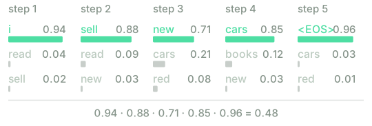
Two vocabularies and an output that stops on its own

Fix two vocabularies: $V_x$ for the input and $V_y$ for the output. The input is a sequence of tokens $x_{1:T_x}$, each $x_j$ an entry of $V_x$. The output is another sequence, $y_{1:T_y}$, over $V_y$, and the two lengths are independent of each other. The encoder is unchanged from the previous lesson: it reads the input from start to finish with the usual recurrence and hands over its last state,

where $\mathbf{o}_{x_j} \in \{0,1\}^{\lvert V_x \rvert}$ is the one-hot vector of the $j$-th token and $\mathbf{W}^{\text{enc}}_{xh} \in \mathbb{R}^{d_h \times \lvert V_x \rvert}$ has one column for each entry of $V_x$. The decoder's recurrence doesn't change either, and it starts where the encoder finished, $\mathbf{s}_0 = \mathbf{c}$. What does change is its output, which now lives in the other language:

with $\mathbf{W}_{hy} \in \mathbb{R}^{\lvert V_y \rvert \times d_h}$, which has one row for each entry of $V_y$ and is the only shape in the model that knows how many entries the target language has. Nothing requires $\lvert V_x \rvert$ and $\lvert V_y \rvert$ to match.

Where the end of the sentence lives

Now for the missing token. To $V_y$, and only to $V_y$, we add one more entry, <EOS>, the end-of-sequence token, and every translation in the training data ends with it: if the correct output has $n$ tokens, the training sequence has $T_y = n + 1$ and its last token is $y_{T_y} = \texttt{<EOS>}$. The loss is the one from the lesson on sequence-to-sequence modelsBlock 3 · Lesson 8Seq2seq: from sequence to sequenceTwo RNNs chained together: an encoder that reads the input sequence and compresses it into a single context vector, and a decoder that writes a new sequence from that vector. The pair trains end to end (the encoder learns only from the gradient the decoder hands back at c) on a toy task that runs in the browser: reversing strings of symbols. It works on short strings and degrades on long ones, because the whole input, whatever its length, has to fit into the same d_h numbers. That bottleneck is the doorway to the next block., unchanged,

and that small piece of bookkeeping is the whole mechanism. The last position sits inside the sum, so it contributes its own term, and gradient descent pushes the probability of <EOS> up exactly there (and, by the same route, down at the earlier positions, where the correct token is a different one). Learning to stop is learning to predict one more token.

That delivers what the task needed: $T_y$ stops being something the loop is handed and becomes something that comes out of the model. When generating, the model writes one token at a time and stops as soon as the token it picks is <EOS>. The code will also have a cap, max_len, so that a badly trained model doesn't write forever. That cap is a safety net in the implementation, not part of the model, and it's worth keeping the two apart.

The decoder defines a distribution over translations

We can write any distribution over sequences, with no assumptions at all, as a product of distributions over one token each. That's the chain rule of probability, applied position by position:

where $y_{<i}$ is the prefix $y_1, \dots, y_{i-1}$: everything written before step $i$. So far there's no architecture at all, since the equality holds for any way of assigning probabilities to sequences. The architecture enters when it decides what each factor gets to look at, and the encoder-decoder's answer is this:

Read it slowly, because the whole block hangs on it. On the left, step $i$ may look at the entire input; on the right, it sees a single vector. Each of the two conditioning terms on the right has a specific home in the model: $\mathbf{c}$ is the initial state $\mathbf{s}_0$, and the prefix $y_{<i}$ is fed back in token by token, so both reach step $i$ already summarised in $\mathbf{s}_{i-1}$. And the factor's probabilities are the coordinates we've already computed: $P(y_i = k \mid y_{<i}, \mathbf{c}) = \hat{y}_{i,k}$.

Generating is walking the product

Writing a translation means choosing a path through those columns. The cheapest path of all takes the largest coordinate at each step,

feeds the chosen token back in and carries on until <EOS>. That's greedy decoding, the same as in the lesson on the character-level language modelBlock 3 · Lesson 7Project: a character-level language modelThe vanilla RNN and BPTT, combined in a network that predicts the next character at every position: a text of T characters is T examples stacked together, and the label at each step comes for free, since it's the character that comes next. It trains with gradient clipping on a few thousand characters (for only a few steps, to fit in the browser) and then writes, feeding back what it samples. The loss falls from ln 26 to around 2.5 and the text goes from noise to broken English (real short words, long near-words, not one sentence that means anything): that's what a character model learns, and saying so outright is the lesson., and it costs one step per output token.

The catch is that this path isn't, in general, the most probable one. Nothing guarantees that the product of the maxima is the maximum of the products: a token that narrowly wins its column can leave the decoder in a state from which everything that follows is bad, and greedy decoding never revisits that decision. Searching for the best path properly would mean scoring $\lvert V_y \rvert^{T_y}$ sentences, which nobody does. Between greedy and exhaustive there are intermediate searches (the usual one is beam search) that this course doesn't cover.

A toy translator in NumPy

Time to train a tiny translator: a toy language with six Spanish words, translated into one with seven English words. It's a toy on purpose (real machine translation doesn't fit in the browser), but it has all three things this lesson has put on the table: two different vocabularies, an output whose length the model decides, and a reordering that forces the model to wait before writing. The Spanish sentences are a verb, a noun and, sometimes, an adjective. Their translation starts with i and moves the adjective in front of the noun. The cell's TO_EN pairs each Spanish word with its English counterpart, so you can read both sides of every pair. Run the cell and look at the pairs.

Compare the two length columns on the right. The translation has one more word than the sentence (the i that Spanish doesn't write), and the sequence the decoder has to produce is one longer still, because <EOS> occupies a position like any other token and has to be predicted too: $T_y = T_x + 2$. There are twelve possible sentences in all, so the model isn't going to learn Spanish; it's going to learn those twelve. It's the mechanism that's on trial, not the translator.

The next cell builds the two networks and trains them. Its train_step is the previous lesson's, line for line: the encoder's forward pass, the decoder's forward pass with teacher forcing, the decoder's backward pass and, hanging off the gradient at $\mathbf{c}$, the encoder's. The only differences are the two vocabularies (nx columns at the input, ny rows at the output) and the <EOS> that sentence already put at the end of every translation.

The loss starts near $\ln 8 \approx 2.08$ (the probability spread evenly over the eight entries of $V_y$, counting <EOS>) and falls almost to zero. Now for the part that matters: generating. The loop below is never given the length of the output. It writes a token, checks whether it was <EOS> and, if so, stops. max_len is there only for safety.

Two things stand out in that table. First, the length columns: two or three tokens go in and three or four come out, always one more, and the model decided that number itself when it placed <EOS> (there's no range(len(x)) anywhere in the loop). Second, the order: when the sentence has an adjective, the model writes it before the noun even though it read it after. To do that it had to hold on to the noun while writing the adjective, and the only thing it had to hold it in was $\mathbf{c}$.

Test your intuition

Four questions: why an end-of-sequence token is needed, exactly which distribution the decoder defines, whether greedy decoding is optimal, and where the ability to stop in the right place comes from.

With the architecture stated precisely, an uncomfortable line comes into view: $P(y_i \mid y_{<i}, x_{1:T_x}) = P(y_i \mid y_{<i}, \mathbf{c})$. That equality isn't a theorem but a design decision, and it claims something strong: that $d_h$ numbers are enough to carry everything the input has to contribute to any position of the output. In a three-token toy nobody would notice. What happens to that claim when the input is a real sentence?

You can measure the answer, and that's what the next lesson, on the context-vector bottleneck, is for. The input keeps getting longer while you watch what happens to the output, until you see where the equality above stops holding and why the breaking point doesn't depend on how much you train.