Project: a sentiment classifier

28 min read

Accuracy over examples the network has already seen isn't a measurement, it's a memory. The previous lesson, on implementing an MLP (multilayer perceptron) from scratch, ended with a loop that trains on its own and a final figure that was never actually at risk: four hand-made examples, and a network with more than enough weights to memorise them outright. What's missing isn't a better loop. It's a text the network has never read, and a number that says what it did with it.

Those two pieces come from different places entirely. The representation was settled a whole block ago: the bag of words turns any text into a fixed-length vector, and does it without anybody having to read the data first. The other piece hasn't shown up in the course at all yet, and it takes up half this lesson: setting a few reviews aside before training even starts, letting them take part in nothing whatsoever, and only asking the network about them once there's nothing left to adjust. With both pieces in place, this is Block 1 feeding the input and Block 2 sitting on top of it, without changing a single line of the loop (checking that is part of the work); the only genuinely new thing is where each piece comes from.

I generated the reviews with artificial intelligence: 240 one-line film reviews, half speaking well of the film and half speaking badly, in the same register as the ten in the lesson on the artificial neuron. That's worth keeping in mind when you read the figure at the end, because a corpus generated this way comes out more regular than one collected off the internet (fewer typos, less irony, a more repetitive vocabulary), and all of that makes the classifier's job easier than it should be. They live in this file, and it's worth opening before reading any further: looking at the data a model is about to train on is part of the work, and here it only takes two minutes. It also holds the split (180 for training, 60 for measuring), written directly into the file rather than drawn at run time, so the numbers below come out identical for you too.

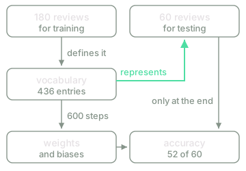
Everything the network learns comes out of the left-hand column. The 60 reviews on the right receive exactly one thing from training (the vocabulary they get represented with) and enter the calculation only once, at the very end, once there's nothing left to adjust.

From the review to the vector, and from there to the network

The input is already fixed by the previous block. Each review is a document $d$ , and its bag of words is the vector counting how many times each vocabulary entry appears in it,

\mathbf{x}_d = \sum_{t=1}^{T_d} \mathbf{o}_{w_t} \in \mathbb{R}^{\lvert V \rvert},

with $T_d$ the number of tokens in the document and $\mathbf{o}_w$ the one-hot of entry $w$ . The vocabulary $V$ is the 436 distinct types appearing in the 180 training reviews, with no frequency cut at all: the lesson on vocabulary and out-of-vocabulary (OOV) words cut at the $k$ most frequent types only because that corpus was large, and here the 180 training reviews add up to no more than 1,359 occurrences total (the first cell below counts them), which isn't enough to justify throwing anything away.

Stack one review per row, and the network's input is $\mathbf{X} \in \mathbb{R}^{N_{\text{train}} \times \lvert V \rvert} = \mathbb{R}^{180 \times 436}$ , with the labels sitting in $\mathbf{Y} \in \mathbb{R}^{180 \times 1}$ , worth $1$ when the review speaks well. On top of it goes the same MLP as the previous lesson, only at different sizes: a hidden layer of $d_1 = 12$ neurons with $\tanh$ and one output with a sigmoid, so $d_0, d_1, d_2 = 436, 12, 1$ . Each step still looks at the whole training set, so $B = N_{\text{train}} = 180$ , and the forward pass takes the usual two lines:

\mathbf{H}^{(1)} = \tanh\left(\mathbf{X}\left(\mathbf{W}^{(1)}\right)^{\top} + \mathbf{1}_B\left(\mathbf{b}^{(1)}\right)^{\top}\right) \in \mathbb{R}^{180 \times 12}, \qquad \hat{\mathbf{Y}} = \sigma\left(\mathbf{H}^{(1)}\left(\mathbf{W}^{(2)}\right)^{\top} + \mathbf{1}_B\left(\mathbf{b}^{(2)}\right)^{\top}\right) \in \mathbb{R}^{180 \times 1}.

The loss is the binary cross-entropy from the lesson on loss functionsBlock 2 · Lesson 5Loss functions: MSE and cross-entropyA loss sums up in one number how badly the network is doing, and between two candidates its derivative is what decides. Mean squared error hands over its smallest correction exactly where the network is wrong with the most confidence; cross-entropy, which comes from reading the output as a probability, leaves that derivative at the plain difference between what was predicted and the label., averaged over the 180 reviews, and the backward pass is the previous lesson's untouched: $\boldsymbol{\Delta}^{(2)} = \hat{\mathbf{Y}} - \mathbf{Y}$ , the recurrence carrying it to the hidden layer, and the four gradients with their $1/B$ ,

\nabla_{\mathbf{W}^{(l)}}\mathcal{L} = \frac{1}{B}\left(\boldsymbol{\Delta}^{(l)}\right)^{\top}\mathbf{H}^{(l-1)}, \qquad \nabla_{\mathbf{b}^{(l)}}\mathcal{L} = \frac{1}{B}\left(\boldsymbol{\Delta}^{(l)}\right)^{\top}\mathbf{1}_B.

The only thing that's actually changed is the sizes, and they've changed enormously: where the four-phrase network had seventeen numbers to adjust, this one has $436 \times 12 + 12 + 12 \times 1 + 1 = 5\,257$ : the weights and biases of the two layers together.

That jump forces one single decision back into view, the scale of the initialisation. Each review lights up roughly seven of the 436 coordinates (the first cell below measures it exactly), so a hidden neuron's pre-activation is a sum of about seven weights: with normal weights at scale $1$ , that produces values large enough to leave the hyperbolic tangent saturated from the very first step, and at scale $0.1$ it doesn't. The difference shows up directly in the result ( $0.700$ accuracy on the new reviews versus $0.867$ ), which is exactly why the cell below multiplies by $0.1$ . That the right scale depends on the width of the layers and the depth of the network is the debt the previous lesson left marked down for Block 3, and it's still there, unpaid.

Measuring where accuracy actually means something

Call $D_{\text{train}}$ the 180 reviews the network trains on and $D_{\text{test}}$ the 60 that get held back, with $N_{\text{train}} = 180$ and $N_{\text{test}} = 60$ . They share no review at all, and that's the entirety of their relationship.

The same figure can be asked of either one, the accuracy: what fraction of its reviews gets the right verdict. The output is a probability, so the verdict counts as positive when $\hat{y}_d \geq 1/2$ (the boundary from the lesson on the artificial neuron) and negative otherwise, giving

\text{accuracy}(D) = \frac{1}{\lvert D \rvert}\left\lvert\left\{\, d \in D \;:\; \hat{y}_d \geq \tfrac{1}{2} \iff y_d = 1 \,\right\}\right\rvert.

The double implication says the two statements carry equal weight: either the network says yes and the label agrees, or neither of them does. And which set gets counted over is written right there inside it, which is exactly what tells $\text{accuracy}(D_{\text{train}})$ apart from $\text{accuracy}(D_{\text{test}})$ , two numbers this lesson is about to look at side by side that don't mean remotely the same thing.

That $V$ comes only out of $D_{\text{train}}$ is part of the measurement itself, not some implementation detail. A vocabulary built over all 240 would give every test review its own coordinate for each of its rare types, coordinates that exist only because that specific review exists, and the network would show up to the exam with the space already cut to its exact measure. What would vanish is exactly what needs measuring: the types a genuinely new text brings that the vocabulary doesn't have. It's the OOV problem from that earlier lesson, arriving here without the safety net that lesson built underneath it: there's no <UNK> to catch these, so a token outside the vocabulary never reaches the vector at all.

This concession needs stating in full, because it has an extreme case. A review whose tokens were all outside the vocabulary would receive $\mathbf{x}_d = \mathbf{0}$ , and with it

\hat{y} = \sigma\left(\mathbf{W}^{(2)}\tanh\left(\mathbf{b}^{(1)}\right) + b^{(2)}\right),

a number that depends not on the review at all, only on the biases: every review this vocabulary can't read gets the exact same verdict, whatever that happens to be. It's the same hole the lesson on the artificial neuron already pointed at, when it looked at what a neuron answers for the null vector, now sitting behind a real piece of text. And a second concession, duller but far more common: sixty reviews measured once give a number with about the reliability of sixty coin tosses, enough to tell a $0.9$ apart from a $0.5$ , but not from a $0.87$ .

The classifier, end to end

The first cell loads the reviews, tokenises them and builds the two matrices. Run it and check three things: the width of the vector, how many of its coordinates are non-zero, and how many test tokens fall through the cracks.

import json, re
import numpy as np
from collections import Counter
from pyodide.http import open_url

D = json.load(open_url("/courses/dl-nlp/resenas-cine.en.json"))
train, test = D["training"], D["test"]


def tokenise(text):                           # the previous block's tokenisation, in one
  return re.findall(r"\w+", text.lower())   # line: down to lower case, punctuation out


freq = Counter(w for r in train for w in tokenise(r["text"]))
V = sorted(freq)                              # the vocabulary comes ONLY from the training set
pos = {e: i for i, e in enumerate(V)}


def matrix(reviews):
  X = np.zeros((len(reviews), len(V)))
  for i, r in enumerate(reviews):
      for token in tokenise(r["text"]):
          if token in pos:                  # what is not in V never reaches the vector
              X[i, pos[token]] += 1.0
  return X, np.array([[float(r["label"])] for r in reviews])


X_train, Y_train = matrix(train)
X_test, Y_test = matrix(test)

print("training:   %d reviews, %d positive" % (len(train), int(Y_train.sum())))
print("test:       %d reviews, %d positive" % (len(test), int(Y_test.sum())))
print("vocabulary: %d entries over %d occurrences" % (len(V), sum(freq.values())))
print("X_train", X_train.shape, "  X_test", X_test.shape)
print("non-zero coordinates: %.1f per review, %.1f %% of the vector"
    % (X_train.astype(bool).sum(1).mean(), 100 * X_train.astype(bool).mean()))

test_tokens = [w for r in test for w in tokenise(r["text"])]
out = [w for w in test_tokens if w not in pos]
print("\nout of vocabulary: %d of %d occurrences (%.1f %%), %d types"
    % (len(out), len(test_tokens), 100 * len(out) / len(test_tokens), len(set(out))))

print("\ntest review:", test[0]["text"])
print("its vector, without the zeros:",
    {V[j]: int(X_test[0, j]) for j in np.nonzero(X_test[0])[0]})

numpy

The first run downloads the Python interpreter (~15 MB). After that it stays in the browser cache and is reused across every lesson.

The three numbers show exactly what the network has got itself into. The vector has 436 coordinates, and a review lights up $7.3$ of them on average, a mere $1.7\%$ : the representation is sparse, as the previous block promised, and every example leaves roughly 429 coordinates saying nothing at all. And of the 455 occurrences in the test set, 23 (that $5.1\%$ , spread across 23 types) aren't in the vocabulary. The last line shows one of them directly: the review a beautiful film that I recommend without reservations reaches the network with only seven coordinates, because reservations shows up in none of the 180 training reviews and vanishes without a trace.

The second cell is the previous lesson's loop with the names changed. It needs whatever the first cell left behind, so run them in order. Watch the last two columns together, since that's really the whole lesson.

import numpy as np

# Needs the previous cell: X_train, Y_train, X_test, Y_test and V.
B, d0, d1, d2 = len(X_train), len(V), 12, 1
eta, steps = 0.5, 600

rng = np.random.default_rng(0)                # fixed seed: you will see these numbers
W1, b1 = rng.normal(size=(d1, d0)) * 0.1, np.zeros(d1)
W2, b2 = rng.normal(size=(d2, d1)) * 0.1, np.zeros(d2)


def output(X, W1, b1, W2, b2):
  H1 = np.tanh(X @ W1.T + b1)
  return H1, 1.0 / (1.0 + np.exp(-(H1 @ W2.T + b2)))


def accuracy(X, Y, W1, b1, W2, b2):
  P = output(X, W1, b1, W2, b2)[1]
  return float(((P >= 0.5) == (Y == 1.0)).mean())


print(" step      loss   training accuracy   test accuracy")
for t in range(steps + 1):
  H1, Y_hat = output(X_train, W1, b1, W2, b2)
  if t % 50 == 0:
      p = np.clip(Y_hat, 1e-12, 1.0 - 1e-12)
      print("%5d   %7.4f   %17.3f   %13.3f"
            % (t, -np.mean(Y_train * np.log(p) + (1.0 - Y_train) * np.log(1.0 - p)),
               accuracy(X_train, Y_train, W1, b1, W2, b2),
               accuracy(X_test, Y_test, W1, b1, W2, b2)))
  if t == steps:
      break
  D2 = Y_hat - Y_train                      # the backward pass, as in the previous lesson
  D1 = (D2 @ W2) * (1.0 - H1 ** 2)
  W1 -= eta * (D1.T @ X_train) / B
  b1 -= eta * D1.sum(0) / B
  W2 -= eta * (D2.T @ H1) / B
  b2 -= eta * D2.sum(0) / B

P_test = output(X_test, W1, b1, W2, b2)[1]
wrong = np.nonzero((P_test >= 0.5) != (Y_test == 1.0))[0]
print("\nit gets %d of the %d test reviews wrong:" % (len(wrong), len(test)))
for i in wrong:
  print("   ŷ = %.3f   y = %d   %s" % (P_test[i, 0], int(Y_test[i, 0]), test[i]["text"]))

numpy

The first run downloads the Python interpreter (~15 MB). After that it stays in the browser cache and is reused across every lesson.

At step $0$ the network answers by coin toss, $0.511$ and $0.550$ , with the loss sitting at $0.6930$ (the $\log 2$ of a network that answers the same thing to everything). By step $100$ it's already right about every review it's looking at, and $0.850$ right about the ones it isn't, and by step $150$ the second column reaches $0.867$ and never lets go again. What's genuinely interesting starts right there: between step $150$ and step $600$ the loss drops by a factor of twelve, from $0.0437$ to $0.0035$ , and the right-hand column doesn't move by a thousandth. Run it for 20,000 steps instead of 600, and it's still sitting at $0.867$ . The eight reviews it gets wrong aren't missed for lack of training.

Read them, since that's where this lesson's real result lives. Four of the eight carry a not. Three speak well of the film and come back negative, I was not bored for a single minute at $0.001$ and it is not bad at all at $0.004$ ; the fourth runs the opposite way and is the sharpest of the set, because the training reviews carry I recommend it to anyone who enjoys good cinema as a positive one, and this test review adds only two more words to it. The other four have nothing to do with negation at all: one loses four of its eight tokens to the vocabulary and arrives as only three coordinates, two lean on entries the training reviews met far more often while speaking well, and the last comes back at $0.511$ , a tie the threshold has to break somehow. The third cell goes after the first four.

import numpy as np

# Needs the two previous cells: tokenise, pos, V, output and the trained weights.
def vector(text):
  x = np.zeros((1, len(V)))
  for token in tokenise(text):
      if token in pos:
          x[0, pos[token]] += 1.0
  return x


def probability(text):
  return float(output(vector(text), W1, b1, W2, b2)[1][0, 0])


a = "the film is not boring, it is fun"
b = "the film is not fun, it is boring"
print("the same vector?", bool(np.array_equal(vector(a), vector(b))))
print("ŷ = %.4f   %s" % (probability(a), a))
print("ŷ = %.4f   %s" % (probability(b), b))

# What can the network know about "not"? Whatever its column says, and its column says this.
n_pos = sum(tokenise(r["text"]).count("not") for r in train if r["label"] == 1)
n_neg = sum(tokenise(r["text"]).count("not") for r in train if r["label"] == 0)
print("\n\"not\": %d occurrences in positive reviews, %d in negative" % (n_pos, n_neg))

# And a review that shares no entry at all with the vocabulary.
new = "sublime filmmaking, essential viewing"
print("\n%s\n   null vector: %s   ŷ = %.4f"
    % (new, not vector(new).any(), probability(new)))

numpy

The first run downloads the Python interpreter (~15 MB). After that it stays in the browser cache and is reused across every lesson.

The first two sentences share the same words, with the same repetitions, in a different order, and they say opposite things. Their vectors turn out identical (the first line confirms it), and so does their probability, $0.0002$ for both: the network calls them both negative, getting one of them right purely by accident. No amount of accuracy can fix that, because the mistake is already locked in before the network ever sees its input.

The second output explains the four failures involving not. That entry appears 5 times in positive training reviews and 20 times in negative ones, so its coordinate ends up pulling towards negative, which is genuinely the best it can do: the coordinate only records how many times not shows up, never what it's actually negating. And the last line closes out the previous section's concession with an actual number: sublime filmmaking, essential viewing shares no entry with the vocabulary at all, receives the null vector, and with it a $0.4140$ that depends on nothing about what it says, only on the biases. Any other unreadable review would get that exact same $0.4140$ , and since it sits below $1/2$ , every one of them would come back negative.

Test your intuition

Three questions: where the vocabulary is allowed to come from, what an OOV rate is actually counted over, and what the gap between the two columns really licenses you to conclude.

This lesson builds its vocabulary out of the 180 training reviews alone. If it were built over the 240, what would be true? Tick everything that holds.

Select every correct option. This is graded all-or-nothing: there is no partial credit.

The test reviews would stop having tokens outside the vocabulary, so the 5.1 % of occurrences that are lost today would disappear from the measurement without having disappeared from the problem.A test review would have coordinates that exist because that same review exists, so the final figure would no longer say what the network does with a text that arrives afterwards.The network would see the labels of the 60 test reviews while it trains.Accuracy over the 180 training reviews would fall, because a larger vocabulary forces more weights to be adjusted with the same examples.

You measure another test set with this same vocabulary. Its reviews come to 500 occurrences of 320 distinct types, and 80 of those types (100 occurrences between them) are not in $V$ . What fraction of that set's occurrences falls outside the vocabulary?

A margin of ±0.005 is accepted.

The network gets the 180 training reviews right and 52 of the 60 test ones. Training it 20,000 steps instead of 600 leaves that second figure exactly where it was. What can be concluded from that?

That the eight it misses are not missed for want of training: the loss goes on falling over the 180 without moving the test accuracy, so whatever separates the two figures is out of reach of the descent.That the descent has fallen into a local minimum, and with another initialisation the network would reach all 60.That the learning rate is too high and the step is skipping over the region where the eight would be put right.That the 60 test reviews are mislabelled, because a network that gets 100 % of what it sees right should not fail on a similar text.

The block ends with a classifier that works, and with the ceiling of its representation in full view. The two sentences in the last cell aren't some contrived case built specifically to make it fail: they follow directly from $\mathbf{x}_d$ summing the one-hots of the tokens, and a sum has no way of remembering what order its summands arrived in. Everything this block has built (the neuron, the layers, the descent, the whole backward pass) operates after that sum happens, and no amount of training can reach back to recover what the input already threw away before it ever existed. That's exactly why the eight reviews hold out against 20,000 steps: it isn't the network that's falling short here.

What's missing, then, is an input that arrives in order and a network able to read it that way, token by token, carrying along whatever it has already seen. That's Block 3, on recurrent neural networks, and its lesson on why the MLP fails with sequences opens by measuring the exact size of the problem: what happens to a multilayer perceptron once the input stops having a fixed length, and the position each token occupies starts to actually mean something.

Was this helpful?