The forward pass in matrix form

The previous lesson, on XOR and hidden layers, left the network complete but unwritten. Complete, because no piece is missing: neurons grouped into layers, each with its own weights and bias, and a $\varphi$ sitting between them that stops the stack from collapsing back into a single neuron. Unwritten, because every pre-activation there was computed on its own, and a pile of loose sums isn't a formula: you can't do algebra with it, and you can't program it as a single thing. The walk from input to output has a name, the forward pass, and one fixed form it's always written in. This lesson is that form.

Put some real numbers on it before writing anything down. Take the ten reviews from the lesson on the artificial neuronBlock 2 · Lesson 1The artificial neuronA weighted sum and a threshold are all a single unit needs to turn a vector into a decision. Its weights sit perpendicular to a boundary that splits the space in two, and the number it computes before deciding measures how far the input has landed from that boundary., with that same eight-entry vocabulary. What goes into the network isn't the review itself but its bag of words: a vector of eight coordinates, one per vocabulary entry, holding how many times that entry shows up in the review. That's all the network ever gets to read. Add a hidden layer of four neurons on top: each one looks at those eight coordinates and returns a number, so the ten reviews together produce $10 \cdot 4 = 40$ hidden pre-activations, each one a sum of eight products plus a bias. Taken one at a time, that's forty separate computations, or two nested loops if you'd rather let the computer grind through them. All forty fit into a single matrix product instead, and the next layer comes out of another product of the same kind. What needs pinning down is what multiplies what, and where the ten reviews actually go in. Because they're going in together: a group of examples running through the network at once is called a batch, and this lesson's batch has ten.

That product isn't shorthand for the two loops: it's the exact same computation, with all the bookkeeping folded into the shapes of the arrays. Look at where each number actually ends up.

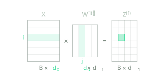
A whole layer in a single product

Fix any layer and call its width $d_l$, the number of neurons it holds. Layer $l$ receives $d_{l-1}$ numbers and hands back $d_l$, so its weights form a matrix $\mathbf{W}^{(l)} \in \mathbb{R}^{d_l \times d_{l-1}}$ and its biases a vector $\mathbf{b}^{(l)} \in \mathbb{R}^{d_l}$, one per neuron. For a single example, the previous lesson already wrote out the result:

with $\mathbf{h}^{(l-1)} \in \mathbb{R}^{d_{l-1}}$, $\mathbf{z}^{(l)}, \mathbf{h}^{(l)} \in \mathbb{R}^{d_l}$, and $\varphi$ applied coordinate by coordinate. The vectors are columns, as they are everywhere in this course, which is why the product is written in that order.

Each layer leans on the one before it, so the chain needs somewhere to start. The first layer has nothing in front of it: what it receives is the raw example, and the convention is to count the input as layer $0$, one that computes nothing at all, $\mathbf{h}^{(0)} = \mathbf{x}$. That makes $d_0$ the dimension of the input, not the width of any actual layer of neurons. For the reviews above, $\mathbf{h}^{(0)}$ is the eight counts of the bag of words, and $d_0 = 8$.

What's worth seeing is that there's nothing new hiding inside that product. Expand the $j$-th coordinate:

That sum is exactly the neuron from the lesson on the artificial neuronBlock 2 · Lesson 1The artificial neuronA weighted sum and a threshold are all a single unit needs to turn a vector into a decision. Its weights sit perpendicular to a boundary that splits the space in two, and the number it computes before deciding measures how far the input has landed from that boundary., with row $j$ of $\mathbf{W}^{(l)}$ playing the role of the weight vector. The matrix product doesn't add any new operation: it groups together the $d_l$ sums that were already there, and all it really contributes is that you never have to write them out one by one. The cost also comes from there: $d_l \cdot d_{l-1}$ products per example, a figure that grows with the size of the layer even though the line of code writing it stays exactly one.

The batch enters from the left, and that is where the transpose comes from

Now bring in the examples. Call the batch size $B$, and store the $B$ examples in a matrix $\mathbf{X} \in \mathbb{R}^{B \times d_0}$, one example per row. That ordering, batch first, is the one this whole course uses, and it's the one NumPy uses too. With the same layout for whatever comes out of each layer, $\mathbf{H}^{(l)} \in \mathbb{R}^{B \times d_l}$, row $i$ of $\mathbf{H}^{(l-1)}$ is example $i$ laid flat: it's $\left(\mathbf{h}^{(l-1)}_i\right)^{\top}$, transposed, because the vector itself is a column and a matrix row is not.

That transpose is the one that propagates through everything else. Transpose the equation above for example $i$, remembering that transposing a product reverses the order of its factors:

which is an equality between two rows: on the left, row $i$ of $\mathbf{Z}^{(l)}$; on the right, row $i$ of $\mathbf{H}^{(l-1)}$ multiplied by that same matrix everyone else uses. Stacking all $B$ rows turns into a single product:

with $\mathbf{Z}^{(l)}, \mathbf{H}^{(l)} \in \mathbb{R}^{B \times d_l}$ and $\mathbf{1}_B \in \mathbb{R}^{B}$ the vector of ones. That last factor deserves its own sentence, since it's the one thing in the formula that never shows up in the code. $\mathbf{Z}^{(l)}$ has $B$ rows and $\mathbf{b}^{(l)}$ has $d_l$ coordinates: adding the two directly isn't even a valid operation between matrices, so what's really written is the product $\mathbf{1}_B\left(\mathbf{b}^{(l)}\right)^{\top}$, the same row of biases repeated $B$ times over. NumPy does that repetition automatically when you write + b, without ever building the matrix, which is exactly why it's worth seeing once what's actually happening underneath.

From input to output, one layer after another

With one layer solved, the network amounts to repeating it. Let $L$ be the number of layers (including the output one), and let $d_0, d_1, \dots, d_L$ be the widths of the chain, starting from the input. The forward pass is this recurrence:

and whatever comes out of the last layer is the network's prediction for all $B$ examples at once, $\hat{\mathbf{Y}} = \mathbf{H}^{(L)} \in \mathbb{R}^{B \times d_L}$. That chain is the entirety of what a multilayer perceptron (MLP) computes: there are no further steps, and nothing later in this block adds any either. What changes from here on is only the numbers sitting inside the matrices.

Two things follow directly from the shapes. The first is the only condition you actually have to respect when designing a network: $\mathbf{H}^{(l-1)}$ has $d_{l-1}$ columns, and $\mathbf{W}^{(l)}$ needs to match, or the product does not exist at all. The intermediate widths are yours to choose; $d_0$ comes from however the input is represented, and $d_L$ from how many answers you want out. The second is that $B$ never appears in a single weight matrix. How many examples run through at once is a decision made by whoever runs the network, not a property of the network itself, and that's where the parameter count comes from:

For the review network below, with $d_0 = 8$, $d_1 = 4$ and $d_2 = 1$, that works out to $41$ numbers. Swap in a vocabulary of $20\,000$ entries and a hidden layer of $128$ neurons instead, and the count jumps to $2\,560\,257$: almost all of it sitting in $\mathbf{W}^{(1)}$, none of it depending on $B$.

The loop, the product and the review network in NumPy

The first cell puts the two versions head to head on a layer of thirty-two neurons: the double loop that follows directly from the definition, and the matrix product. Run it and check three things: whether the two agree, how long each one actually takes, and what happens when the product is written without transposing.

The two versions produce the same numbers: the largest difference the cell prints out is $0$. But getting there doesn't cost the same at all: the product runs between one and two orders of magnitude faster, and the exact factor depends on the machine and the browser you're using. Where that speed-up comes from doesn't depend on either one, though. It's not that the product performs fewer operations (it does exactly the same number), but that Python works through the $4\,096$ turns of the loop one at a time, while the product runs them inside a compiled routine that never goes back through the interpreter.

The last two experiments are the two classic shape traps. X @ W doesn't exist, and NumPy tells you so by naming the exact two dimensions that fail to line up; and the difference between $\mathbf{Z}$ and the product without a bias comes out to the same triple, $-0.761$, $3.221$, $0.221$, in both row $0$ and row $127$, which is $\mathbf{1}_B\mathbf{b}^{\top}$ made visible.

The second cell builds the whole network over the ten reviews: eight vocabulary entries, four hidden neurons with ReLU (rectified linear unit), and one output neuron with a sigmoid, so what it hands back is a number between $0$ and $1$. Run it and pay attention to the column of shapes, and to the last line.

Five lines of code for the entire network, and the reason is right there in the column of shapes: the $10$ in the first dimension never gets touched anywhere and arrives at the end fully intact, while the second dimension keeps changing, $8 \to 4 \to 1$, in step with the widths. The network carries exactly the $41$ parameters the count above predicted.

And now the last line, the one that actually matters. Five correct out of ten. Every single output sits below $0.5$ (the highest is $0.485$, for i recommend it), so the network answers no to all ten reviews and happens to get the five negative ones right. That's the score of someone who reads nothing at all and always says no. The weights came straight out of np.random.randn, and there was never any reason to expect otherwise.

Test your intuition

Three questions (how many numbers a network actually stores, where the transpose comes from, and what the chain guarantees), plus a challenge that's the entire forward pass.

The network can now answer, whether you feed it one example or a thousand, and what it answers is worthless. Those two facts fit together perfectly, because the forward pass carries no notion of correctness at all: it's a chain of products that turns $\mathbf{X}$ into $\hat{\mathbf{Y}}$, and it would run exactly the same way with the right weights, if anyone actually knew what they were. Correcting the weights means measuring them first, and measuring isn't the same as counting correct answers. The tally on the last line scores exactly the same whether the output is $0.499$ or $0.036$, and it doesn't budge when a weight shifts slightly: it can't tell apart being wrong by a hair from being wrong completely, and that distinction is the only thing that could actually tell you which way to move a weight.

What's needed is a number that can tell them apart. A single number for the whole batch, one that grows as $\hat{\mathbf{Y}}$ drifts away from the labels, falls as it moves closer, and changes continuously enough to actually have a derivative. How that number gets built, why the first candidate most people reach for (squaring the difference) is the right call for some tasks and a bad idea for classification, and what takes its place instead, is the next lesson, on loss functions: mean squared error and cross-entropy.